Signal compression

We are going to transform a discrete finite signal, a vector, into another containing many zeros and similar information. This is of course easy to store and allows to compress the signal (see Huffman trees and dictionary methods). The idea is to apply a transform to the signal, in our case the Discrete Cosine Transform (DCT) or the Discrete Wavelet Transform (DWT), and set to zero all the absolute values below a certain threshold. This is the signal with many zeros to be stored. With the inverse transform we recover an approximation of the original signal. The procedure works finely when the signal has certain regularity assuring the decay of the transform. The choice of the threshold here depends on the relative energy leak we permit (see my course on signal processing).

In the code below the function compw has as input the signal x, the allowed relative energy loss a and a code to select the transform: 1 for the DCT, 4 for the DWT with D4 and 8 for the DWT with D8. We abbreviate these wavelet transforms as DWT4 and DWT8. The output is the reconstruction of the signal y, the number of zeros nz, the threshold thr, the maximal absolute error linf and the norm of the difference l2. The main code stores the data got from compw in a text data file to produce figures with this sagemath plotter.

For \(N=512\) we consider the signal with \(x_n=-n/N\) for \(0\le n\le N/2\) and \(x_n=1-n/N\) for \(N/2< n< N\). When normalizing the horizontal axis to [0,1], as we do in the following figures, the signal is a discretization of the broken line composed by a segment joining (0,0) to (1/2,-1/2) and another segment joining (1/2,1/2) and (1,0).

The energy scales quadratically and then the aspect of the reconstruction is very sensitive to the value of a. Roughly speaking, the norm error is proportional to its square root. This means that a must be very small in practice.

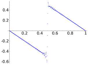
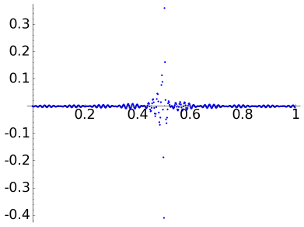
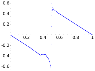
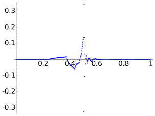
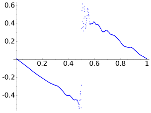
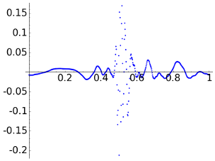
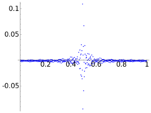
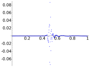
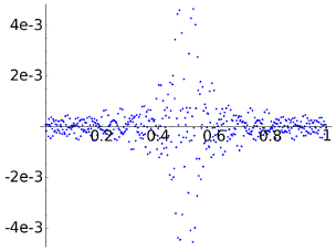
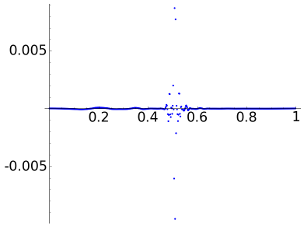
Let us start taking a=1e-2. Although it may sound as a small number, it is not in this context. The figures to the left are the reconstructions and the figures to the right the point error.

DCT
DWT4
DWT8

Moreover, the code gives the following table for the output:

	DCT	DWT4	DWT8
`nz`	396	502	495
`thr`	5.9224e-02	5.2832e-01	3.3063e-01
`linf`	4.1048e-01	3.4170e-01	2.1220e-01
`l2`	6.5121e-01	6.4544e-01	6.4213e-01

The norm of the difference is comparable in any case, as it must to be because a is fixed (to say the whole truth, due to the discretization not always they are so close). This norm error and the maximal absolute error are smaller for the DWT8 but most of us would agree saying that the DCT gives a more faithful intuition about the aspect of the signal. Our sight does not interpret correctly the \(\ell^\infty\) and the \(\ell^2\) norm and we find a difference between our intuition and the mathematical model. To give some support to this model, note that the DWT8 gives a better treatment of the discontinuity, near it the DCT reaches errors beyond 0.3.

If you buy that in some mathematical sense the reconstructions with the DCT and DWTs have comparable errors and even the DWTs give a better approximation, then the first row of the table proves that the DWTs are much better for compression. Note that to reconstruct the signal with the DCT we need 512-177=335 nonzero coordinates out of N=512, this is like a 65.4% while using the DWT4 we only need 10, like a 2.0%. This is quite impressive!

If we reduce the value of a then the reconstruction becomes quite good and any disagreement between the mathematical model and what we consider the aspect of the result is less relevant. The drawback of using smaller values of a is that necessarily the number of nonzero coordinates increases reducing the performance and hence the possibility of compression. In our case this is not so critical and we can safely take a value like a=1e-5 getting a good approximation and a lot of zero coordinates with the DWTs while the DCT is almost useless to compress the signal.

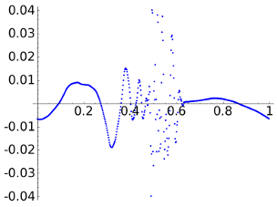
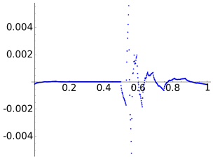
Before checking that example, we take the intermediate case a=1e-3 that produces

DCT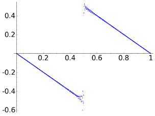
DWT4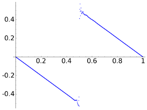
DWT8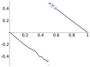

and the table

	DCT	DWT4	DWT8
`nz`	177	498	487
`thr`	2.5603e-02	1.2941e-01	1.1141e-01
`linf`	1.0908e-01	8.6978e-02	4.0057e-02
`l2`	2.0505e-01	1.6775e-01	2.0122e-01

Again, although the last two rows of the table claim that the mathematical measure of the error with the max norm and the 2-norm supports a better reconstruction with the DWTs, probably many people would disagree. It is illustrative to look the scale of the figures showing the error. With respect to the compression, note the dramatic change in the number of zero coordinates of the DCT which has reduced to less than one half while for the DWTs it remains more or less the same.

Finally, let us consider a=1e-5 that gives a quite good reconstruction in every case.

DCT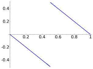
DWT4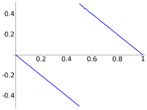
DWT8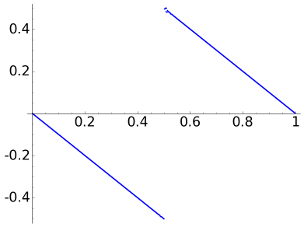

The corresponding table is:

	DCT	DWT4	DWT8
`nz`	36	492	479
`thr`	5.7502e-03	2.4744e-02	2.4298e-02
`linf`	4.6497e-03	5.5927e-03	9.5481e-03
`l2`	2.0183e-02	1.6624e-02	9.5481e-03

Note that the number of nonzero coordinates for the DCT is 476, like 93.0% of the total. On the other hand for the DWT4 this proportion is 3.9% and for the DWT8, it is 7.0%.

The code

This is octave code that produces the figures and the data for the tables:


pkg load signal



clear all





filename = "data_plot.txt";

fid = fopen (filename, "w");



% SIGNAL

N = 512;

t = ( [0:N-1]/N )';

%x = (t<0.5).*(sin(2*pi*t)).^2.*cos(60*pi*t.^2);

%x += (t>=0.5).*sin(5*pi*t)*4.*(1-t).^2;



%z = x + sin(64*2*pi*t)/100;





xx = -1-t-floor(-t-0.5);



metadat = '>!_!_!_\nPJ0 SI%d FI./file_%s.png\n!_!_!_<\n';





% Reconstruction



ths = xx;



a = 1e-2;



for a = [1e-2,1e-3,1e-5]

  if a ==1e-2

    s2 = '_2';

  elseif a ==1e-3

    s2 = '_3';

  elseif a ==1e-5

    s2 = '_5';

%  else

%    s2 = '_6';

  end

  printf('========= %s\n',s2)    

  for c = [1,4,8]

    if c ==1

      s1 = 'dct';

    elseif c==4

      s1 = 'd4';

    else

      s1 = 'd8';

    end

    [zrec, nz, thr, linf, l2] = compw(ths, a, c );

    printf('%s\n',s1)    

    printf('nz = %d\n',nz)

    printf('thr = %.4e\n',thr)

    printf('linf = %.4e\n',linf)

    printf('l2 = %.4e\n',l2)

    printf('---------------\n')





    %fprintf (fid, '(%f, %f)\n', [t'; ths']);

    %fprintf (fid, '>!_!_!_\nPJ0 SI4 ZO1 COred\n!_!_!_<\n');

    st = strcat(s1,s2);

    fprintf (fid, '(%f, %f)\n', [t'; zrec']);

    fprintf (fid, sprintf(metadat,6,st));



    st = strcat(st,'e'); 

    fprintf (fid, '(%f, %f)\n', [t'; (ths-zrec)']);

    fprintf (fid, sprintf(metadat,10,st));

  end

end







fclose (fid);

The two functions referenced in this code are:

compw

thr_ener


 

% Reconstruction of signal: 

% INPUT:

%     x = signal

%     a = relative energy leak

%     c = code transform

% OUTPUT:

%     y = reconstructed signal

%     nz = number of zeros

%     thr = threshold

%     linf = maximal absolute error

%     l2 = mean square error







function [y, nz, thr, linf, l2] = compw(x, a, c )

  N = size(x,1);

  

  if c ==1

    W = dct( eye(N) );

  elseif c==4

    fd4 = [ 1-sqrt(3), sqrt(3)-3, 3+sqrt(3), -1-sqrt(3)]/4/sqrt(2);

    W = wav_tr( fd4, eye(N));

  elseif c==8

    fd8 = [0.32580343 , 1.01094572 , 0.89220014, -0.03957503 , -0.26450717 , 0.0436163 , 0.0465036, -0.01498699];

    fd8 = -fliplr(fd8)/sqrt(2).*(-1).^[1:size(fd8,2)];

    W = wav_tr( fd8, eye(N));

  else

    disp('ERROR, wrong code for the transform')

  end



  u = W*x;

  thr = thr_ener( u, a);

  u = u.*(abs(u)>=thr);

  nz = nnz(~u);

  y = W'*u;

  linf = max(abs(x-y));

  l2 = norm(x-y);

end


 

% threshold from the energy loss: v = signal,  alph = energy loss



function th = thr_ener( v, alph )

  v = sort( abs(v), 'descend');

  z = cumsum( v.^2/norm(v)^2 );

  indx = find( z > 1- alph, 1 );

  th = abs(v(indx));

end

Note also that there is a call to wav_tr