With the normalization as in my signal processing course, the Discrete Wavelet Transform (DWT) is a unitary linear operator on the N dimensional space. Hence it has an N dimensional unitary matrix.
We consider here the cases Haar (D2), D4 and D12, coming from the filters [0.70711, -0.70711], [-0.12941, -0.22414, 0.83652, -0.48296] and [-1.0773e-03, -4.7773e-03, 5.5384e-04, 3.1582e-02, 2.7523e-02 -9.7502e-02, -1.2977e-01, 2.2626e-01, 3.1525e-01, -7.5113e-01, 4.9462e-01 -1.1154e-01].
Given a filter f, the function wav_tr computes the DWT of a signal vector or of a collection of them. In particular, wav_tr( fd4, eye(N)) gives the matrix of the DWT.
DISCLAIMER: It is clear revising the code that this is not an efficient way of computing this matrix because it disregards the internal structure indicated below. The code has only academic purposes. I intended to write something quick, versatile and easy to understand.
With the octave code below we get that using the Haar filter the matrix for N=4 is
0.50000
0.50000
0.50000
0.50000


0.50000
0.50000
-0.50000
-0.50000


0.70711
-0.70711
0.00000
0.00000


0.00000
0.00000
0.70711
-0.70711
N=8 it is
0.35355
0.35355
0.35355
0.35355
0.35355
0.35355
0.35355
0.35355


0.35355
0.35355
0.35355
0.35355
-0.35355
-0.35355
-0.35355
-0.35355


0.50000
0.50000
-0.50000
-0.50000
0.00000
0.00000
0.00000
0.00000


0.00000
0.00000
0.00000
0.00000
0.50000
0.50000
-0.50000
-0.50000


0.70711
-0.70711
0.00000
0.00000
0.00000
0.00000
0.00000
0.00000


0.00000
0.00000
0.70711
-0.70711
0.00000
0.00000
0.00000
0.00000


0.00000
0.00000
0.00000
0.00000
0.70711
-0.70711
0.00000
0.00000


0.00000
0.00000
0.00000
0.00000
0.00000
0.00000
0.70711
-0.70711
For D4 with N=4, the matrix is
0.48296
0.83652
0.22414
-0.12941


0.22414
-0.12941
0.48296
0.83652


-0.12941
-0.22414
0.83652
-0.48296


0.83652
-0.48296
-0.12941
-0.22414
The matrix for D4 with N=4 is
0.20425
0.42075
0.51226
0.63726
0.29575
0.07925
-0.01226
-0.13726


0.29575
0.07925
-0.01226
-0.13726
0.20425
0.42075
0.51226
0.63726


-0.17075
-0.04575
-0.13726
-0.17075
0.35377
0.72877
-0.04575
-0.51226


0.35377
0.72877
-0.04575
-0.51226
-0.17075
-0.04575
-0.13726
-0.17075


-0.12941
-0.22414
0.83652
-0.48296
0.00000
0.00000
0.00000
0.00000


0.00000
0.00000
-0.12941
-0.22414
0.83652
-0.48296
0.00000
0.00000


0.00000
0.00000
0.00000
0.00000
-0.12941
-0.22414
0.83652
-0.48296


0.83652
-0.48296
0.00000
0.00000
0.00000
0.00000
-0.12941
-0.22414
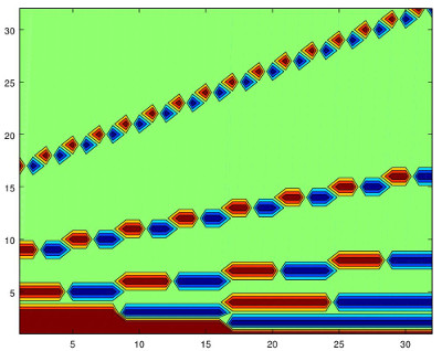
To visualize the situation in higher dimensions, let us consider a contour plot of the matrix for N=32. Dark blue are small values and dark red large values and the number of levels is 6. To prevent the large values of the last rows to mask other values, we normalize each row dividing by the maximum absolute value. In this way, every entry has absolute value at most 1 and each row contains a 1 or -1.
This is the result for the Haar filter:
|
The last rows (second coordinate large) correspond to the upper part. There are 5 levels of ’self-similarity’. The last one with horizontal bands covering one half of the width (imagine that the lower thin line coming from the first row is not there).
For the D4 filter we observe a funnier contour plot:
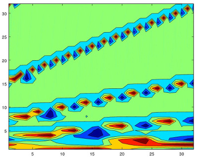 |
The different scales of shifted wavelets correspond according to the cascade algorithm to the rows (2,4], (4,8], (8,16] and (16, 32] but the ’self-similarity’ is more difficult to appreciate.
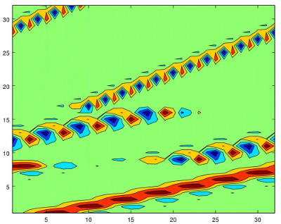
To show that the first rows have a different behavior because they correspond to the scaling function, let us consider the filter D12. Its length is 12 and then we have 8 rows, the least power of two less than 12, giving approximations of shifts of the scaling function. Note that this is reflected in the contour plot:
 |
Just for your curiosity, if we do not normalize the rows, the last contour plot becomes
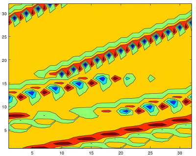 |
Note that we have lost levels in the lower part because the large values in the upper part force to spread them out.
This is octave code that produces the matrices and the figures:
pkg load signal


clear all

%close all


% Haar

haar = [1,-1]/sqrt(2);


% D4

fd4 = [ 1-sqrt(3), sqrt(3)-3, 3+sqrt(3), -1-sqrt(3)]/4/sqrt(2);


% D12 (the bizarre ordering compensated by fliplr is to copy the data from wikipedia)

fd12 = [0.15774243 , 0.69950381 ,1.06226376 , 0.44583132, -0.31998660, -0.18351806 , 0.13788809 , 0.03892321 , -0.04466375 , 7.83251152e-4, 6.75606236e-3, -1.52353381e-3 ];

fd12 = -fliplr(fd12)/sqrt(2).*(-1).^[1:size(fd12,2)];


% SINGLE MATRICES

disp('---Haar N=4---')

disp(wav_tr( haar, eye(4)))


disp('---Haar N=8---')

disp(wav_tr( haar, eye(8)))


disp('---D4 N=4---')

disp(wav_tr( fd4, eye(4)) )


disp('---D4 N=8---')

disp(wav_tr( fd4, eye(8)) )


% NORMALIZED MATRIX OF THE DWT

N = 32

lev = 6

W2 = wav_tr( haar, eye(N));

W4 = wav_tr( fd4, eye(N));

W12 = wav_tr( fd12, eye(N));

W2n = diag(1./max(abs(W2')))*W2;

W4n = diag(1./max(abs(W4')))*W4;

W12n = diag(1./max(abs(W12')))*W12;


% CONTOUR PLOTS

figure(1)

colormap ("default");

contourf (W2n, lev)

print -djpg file1.jpg


figure(2)

colormap ("default");

contourf (W4n, lev)

print -djpg file2.jpg


figure(3)

colormap ("default");

contourf (W12n, lev)

print -djpg file3.jpg


figure(4)

colormap ("default");

contourf (W12, lev)

print -djpg file4.jpg
The functions that compute the matrix of the DWT are (recall the disclaimer):
|
|
wav_tr_m
|
% Wavelet transform: f=filter x=signal |
% Wavelet transform: f=filter x=signal |