Denoising with wavelets

Let us consider a finite discrete signal, represented by a vector ${\mathbb{C}}^N$ with $N$ a power of two, affected by Gaussian noise $N(0,\sigma )$. If the signal is in some sense smooth, its Discrete Wavelet Transform (DWT) should show a quick decay and the noise reappears in the DWT side separating randomly the values from zero. Then a natural idea to denoise the signal is to choose a threshold $\lambda >0$ and set to zero any coordinate of the detail vectors with absolute value less than $\lambda$. This is in fact a general idea that also works with the DFT and other transforms. In the case of the DWT, after the work of Donoho and Johnstone, a good asymptotic choice of the threshold parameter is $$\lambda =\sigma \sqrt{2\log N}.$$

In many practical situations $\sigma$ is unknown. Orthogonal maps transform Gaussian distributed vectors into vectors with the same distribution then we expect the coordinates of ${\overrightarrow{d}}_1$ to be a sample of a distribution $N(0,\sigma )$ except for some outliers corresponding to discontinuities. Due to the possible existence of these outliers we need a very robust estimator and the sample standard deviation is not. A much better option is the median absolute deviation defined as $$\text{MAD}(\{v_n{\}}_{n=0}^{N-1})=\text{median}(|v_0-m|,\dots ,|v_{N-1}-m|)\text{with}m=\text{median}(v_0,\dots ,v_{N-1}).$$ It can be proved that if $\{v_n{\}}_{n=0}^{N-1}$ is a sample of a distribution $N(0,\sigma )$ then one has the convergence in probability $$\text{MAD}(\{v_n{\}}_{n=0}^{N-1})\to K_0\sigma \text{with}{K}_0\approx 0.6745.$$ Using this with $\overrightarrow{v}={\overrightarrow{d}}_1$, the choice of the threshold parameter becomes $$\lambda =\approx 2.0967\text{MAD}({\overrightarrow{d}}_1)\sqrt{\log N}.$$

The octave code below applies this denoising method with the DWT corresponding to different Daubechies wavelets and produces the examples shown here. Note that it calls to a function in "The matrix of the DWT". The output is treated with this sagemath plotter to get the images.

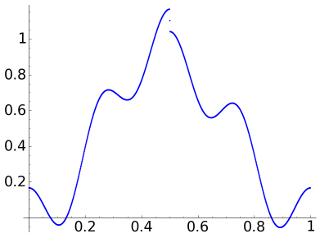
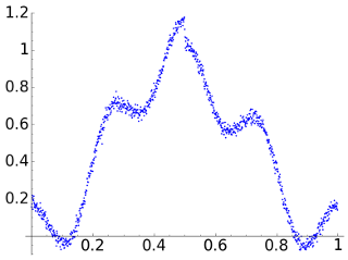
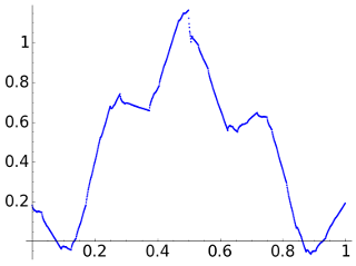
The chosen signal (taken from my course on signal processing) is $\overrightarrow{x}=\{x_n{\}}_{n=0}^{N-1}$ with $N=1024$ given by the following formula where $t=n/N$: $$x_n=\frac{15-\text{sgn}(t-1/2)}{16}{\sin }^2(\pi t)+\frac{1}{6}\cos (8\pi t).$$ We consider it affected by Gaussian noise with $\sigma =0.02$. These are the corresponding plots:

Signal $\overrightarrow{\mathsf{x}}$	Noisy signal $\sigma \mathsf{=}\mathsf{0.02}$

The jump in the discontinuity is $1/8>2\sigma$ then the noise in principle should not mask completely the discontinuity although visually one tends to see the noisy image as coming from a continuous function.

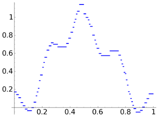
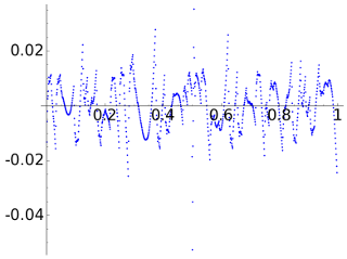
For D2, the Haar wavelet, the graphs of the denoised signal and of the error are

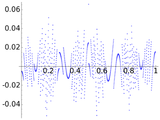Of course the technique for D2 has only an academic interest.

For D4 the result is a little ’shaky’ due to the lack of smoothness of the wavelet. On the other hand the discontinuity has been detected.

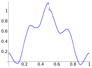
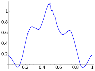
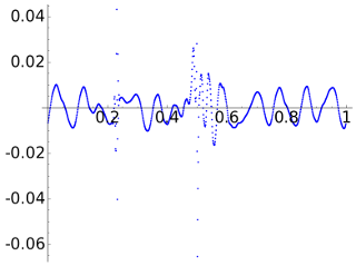
With D8 we get a better result and in general smaller errors except for points very close to the discontinuity which now visually is less obvious.

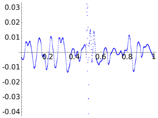Finally, with D12 the error near the discontinuity boosts and there is also a replica, coming from ${\overrightarrow{d}}_2$, that creates a strange spot around $1/4$.

The code

This is octave code that produces the figures:

It requires the functions: