The square wave, the sawtooth wave, the triangle wave and the rectified cosine, are four basic 1-periodic waves with explicit Fourier series. The names are self-explanatory except perhaps in the last case in which the rectification consists in taking the positive part.
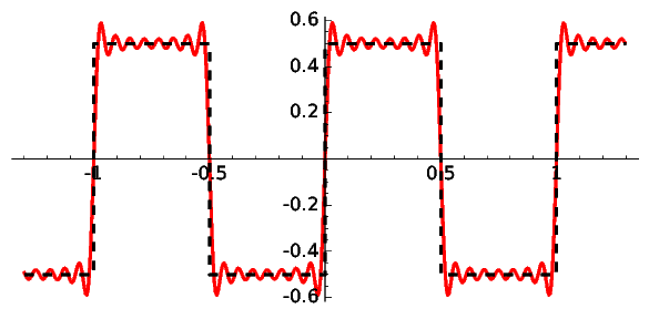
A closed formula for the square wave and its explicit Fourier series are \[\textrm{sq}(t)=\frac{1}{2}(-1)^{\lfloor 2t \rfloor} \qquad \text{and}\qquad \frac{2}{\pi} \sum_{n=1}^\infty \frac{\sin\big(2\pi(2n-1)t\big)}{2n-1}\] where \(\lfloor x\rfloor\) denotes the integral part of \(x\). This is the approximation that we get taking frequencies less than 16:
|
This figure and the rest of the graphs have been plotted with this code.
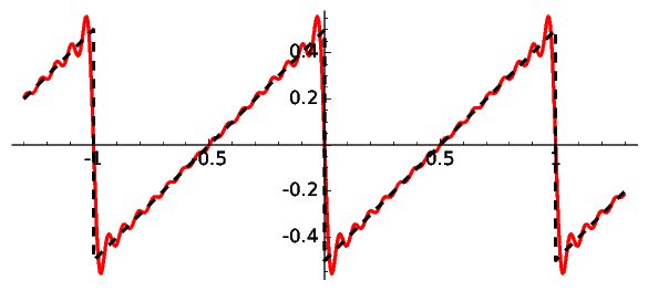
For the sawtooth wave, \[\textrm{st}(t)=t-\lfloor t \rfloor-\frac 12 \qquad \text{and}\qquad -\frac{1}{\pi} \sum_{n=1}^\infty \frac{\sin(2\pi nt)}{n}.\] The approximation considering frequencies less than 16 is:
 |
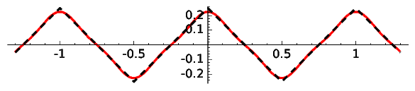
The triangle wave and the rectified cosine are more regular, with frequencies less than 16 we would get something difficult to distinguish from the original. Even taking very few terms in the Fourier series we get a fairly good approximation.
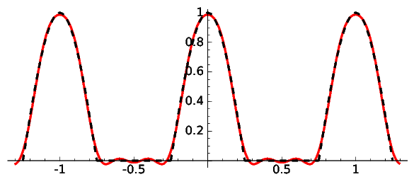
For the triangle wave, the formulas are \[\textrm{tr}(t)=\frac 14 -\big|t-\lfloor t +\frac 12\rfloor\big| \qquad \text{and}\qquad \frac{2}{\pi^2} \sum_{n=1}^\infty \frac{\cos\big(2\pi (2n-1)t\big)}{(2n-1)^2}.\] And for the rectified cosine \[\textrm{rc}(t)=\max\big(0,\cos(2\pi t)\big) \qquad \text{and}\qquad \frac{\cos(2\pi t)}{2} -\frac{1}{\pi}\sum_{n=-\infty}^\infty \frac{(-1)^n\cos(4\pi nt)}{4n^2-1}.\]
Taking only two terms in the case of the triangle wave (it corresponds to frequency at most 3) we get
 |
In the case of the rectified cosine for frequencies at most 4, corresponding to four cosines, we obtain the approximation
 |
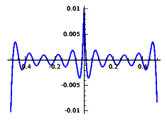
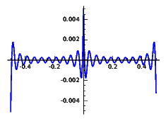
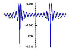
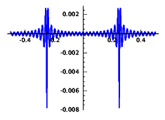
In both cases it is more illustrative to plot the absolute error. Here we consider frequencies at most 10, 20 and 40. Note the vertical scale.
Error for the triangle wave:
 |
 |
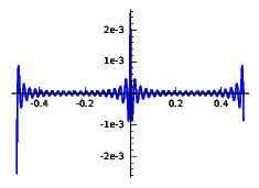 |
| \(F\le 10\) | \(F\le 20\) | \(F\le 40\) |
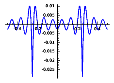
Error for the rectified cosine:
 |
 |
 |
| \(F\le 10\) | \(F\le 20\) | \(F\le 40\) |
The similarity of the latter figures with a shifted reversed plot of the Dirichlet kernel is not by chance. The key to understand this phenomenon is that \((-1)^n\cos(4\pi nt)\) becomes \(\cos(2\pi nu)\) under the change \(t=(2u+1)/4\).
This is the SAGE code to plot the figures.
npoints = 500

th = 2


def mplot( f, co, bb ):

  L = []

  for t in srange(-bb, bb, 2*bb/npoints):

    L.append( (t, f(x=2*pi*t) ) )

  return L


##############

# SQUARE

def sq_w(F, co,fos=16):

  f = 0

  k = 1

  while 2*k-1 <=F:

    f += sin( (2*k-1)*x )/(2*k-1)

    k += 1

  f = 2/pi*f


  L = mplot(f, co, 1.3)[:]

  P = list_plot(L, plotjoined=True, thickness=th, color=co)


  g = 1/2*(-1)^(floor(2*x))

  P += line([(-bb,-1/2), (-1, -1/2), (-1, 1/2), (-1/2, 1/2), (-1/2, -1/2), (0, -1/2), (0, 1/2), (1/2, 1/2), (1/2, -1/2), (1, -1/2), (1, 1/2), (bb,1/2)], linestyle='--', thickness=th, zorder=20, color='black')


  P.fontsize(fos)

  P.set_aspect_ratio(1)

  return P


##############

# SAWTOOTH

def st_w(F, co, fos=16):

  f = 0

  k = 1

  while k <=F:

    f += sin( k*x )/k

    k += 1

  f = -1/pi*f


  L = mplot(f, co, 1.3)[:]

  P = list_plot(L, plotjoined=True, thickness=th, color=co)


  g = x-floor(x)-1/2

  P += line([(-bb,g(x=-bb)), (-1, 1/2), (-1, -1/2), (0, 1/2), (0, -1/2), (1, 1/2), (1, -1/2), (bb,g(x=bb))], linestyle='--', thickness=th, zorder=20, color='black')


  P.fontsize(fos)

  P.set_aspect_ratio(1)

  return P


##############

# TRIANGLE

def tr_w(F, co, fos=16):

  f = 0

  k = 1

  while 2*k-1 <=F:

    f += cos( (2*k-1)*x )/(2*k-1)^2

    k += 1

  f = 2/pi^2*f


  L = mplot(f, co, 1.3)[:]

  P = list_plot(L, plotjoined=True, thickness=th, color=co)


  g = 1/4 -abs(x-floor(x+1/2))

  P += line([(-bb,g(x=-bb)), (-1, g(x=1)), (-0.5, g(x=-0.5)), (0, g(x=0)), (0.5, g(x=0.5)), (1, g(x=1)), (bb, g(x=bb))], linestyle='--', thickness=th, zorder=20, color='black')


  P.fontsize(fos)

  P.set_aspect_ratio(1)

  return P


##############

# ERROR TRIANGLE

def tr_we(F, co, fos=16):

  f = 0

  k = 1

  while 2*k-1 <=F:

    f += cos( (2*k-1)*x )/(2*k-1)^2

    k += 1

  f = 2/pi^2*f

  f = 1/4 - abs_symbolic(x/2/pi) -f


  L = mplot(f, co, 0.5)[:]

  P = list_plot(L, plotjoined=True, thickness=1, color=co)


  P.fontsize(fos)

  return P


##############

# RECTIFIED COSINE

def rc_w(F, co, fos=16):

  f = 0

  k = 1

  while 2*k <=F:

    f += (-1)^k*cos( 2*k*x )/(4*k^2-1)

    k += 1

  f = cos(x)/2-1/pi*(-1+2*f)


  L = mplot(f, co, 1.3)[:]

  P = list_plot(L, plotjoined=True, thickness=th, color=co)


  g = cos(2*pi*x)

  for k in srange(5):

    if is_even(k):

      P += plot( g, x, -5/4+k/2, -3/4+k/2, linestyle='--', thickness=th, zorder=20, color='black')

    else:

      P += line([(-3/4+(k-1)/2,0), (-1/4+(k-1)/2,0)], linestyle='--', thickness=th, zorder=20, color='black')


  P.fontsize(fos)

  P.set_aspect_ratio(1)

  return P


##############

# ERROR RECTIFIED COSINE

def rc_we(F, co, fos=16):

  f = 0

  k = 1

  while 2*k <=F:

    f += (-1)^k*cos( 2*k*x )/(4*k^2-1)

    k += 1

  f = cos(x)/2-1/pi*(-1+2*f)


  f = max_symbolic(0,cos(x)) -f


  L = mplot(f, co, 0.5)[:]

  P = list_plot(L, plotjoined=True, thickness=1, color=co)


  P.fontsize(fos)

  return P


P = sq_w(15, 'red', 12)

#P.save('./file.eps', figsize=6)


P = st_w(15, 'red', 12)

#P.save('./file.eps', figsize=6)


P = tr_w(3, 'red', 12)

#P.save('./file.eps', figsize=6)


P = rc_w(4, 'red', 12)

#P.save('./file.eps', figsize=6)


P = tr_we(10, 'blue', 6)

#P.save('./file.eps', figsize=2.5)


P = tr_we(20, 'blue', 6)

#P.save('./file.eps', figsize=2.5)


P = tr_we(40, 'blue', 6)

#P.save('./file.eps', figsize=2.5)


P = rc_we(10, 'blue', 6)

#P.save('./file.eps', figsize=2.5)


P = rc_we(20, 'blue', 6)

#P.save('./file.eps', figsize=2.5)


P = rc_we(40, 'blue', 6)

#P.save('./file.eps', figsize=2.5)