Rectangular, \(N=20\)
According to the theory, to design a digital low-pass filter with a window determined by the real weights \(w_k\), we have to convolve with \(w_k\,\text{sinc}(2\nu_ck)\) where \(\nu_c\) is the cut frequency and, as usual, \(\text{sinc}(x)\) is \(\sin(\pi x)/(\pi x)\), the Fourier transform of the of the characteristic function of \([-1/2, 1/2]\). In a formula (see my signal processing course), \[x_n\longmapsto y_n, \qquad y_n= 2\nu_c\sum_{k=-N}^N w_k \,\text{sinc} (2\nu_c k) x_{n-k}.\]
With the code below we are going to check how good is this approximation for two values of \(N\) and the rectangular, Hann, Hamming and Blackman (exact) windows. For the attenuation in decibels with these windows see this. We normalize the situation to a sampling frequency \(\nu_s=1\) (Nyquist frequency \(1/2\)) and then the positive range of frequencies is \(0\le \nu<1/2\).
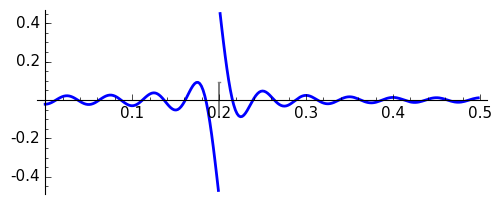
If we naively consider the error in the approximation as the difference in \([0,1/2)\) of the \(2\nu_c\sum_{k=-N}^N w_k \,\text{sinc} (2\nu_c k) \cos(2\pi k\nu) \) and the characteristic function of \([0,\nu_c)\), then we have a big error term near \(\nu_c\) because we are subtracting a smooth function from a discontinuous one. For instance, for the rectangular window with \(N=20\) the graph of this error is:
| |
|
Rectangular, \(N=20\)
|
Of course we need to separate the transition band. In the code I have taken as mathematical definition of the extremes of the transition band the last zero in the error for the left part and the first zero in the error for the right part.
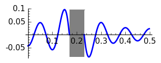
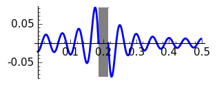
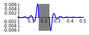
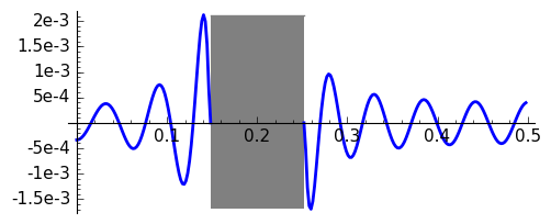
Running the program one gets the following graphs of the error for \(N=10\) and \(N=20\) where the gray rectangle corresponds to the transition band.
 |
 |
|
Rectangular, \(N=10\)
|
Rectangular, \(N=20\)
|
 |
 |
|
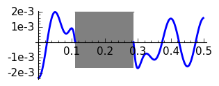
Hann, \(N=10\)
|
Hann, \(N=20\)
|
 |
 |
|
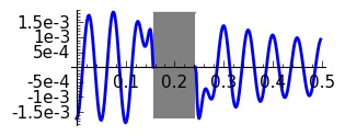
Hamming, \(N=10\)
|
Hamming, \(N=20\)
|
 |
 |
|
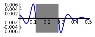
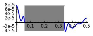
Blackman, \(N=10\)
|
Blackman, \(N=20\)
|
The graphs are coherent with the theory. Note that doubling \(N\) the transition band approximately reduces a 50% its width. The rectangular window has the thinnest transition band but the Gibbs phenomenon produces an unavoidable error of approximately 0.09. The motivation for introducing windows is in fact to reduce Gibbs phenomenon at the cost of enlarging the transition band. Then Hann and Hamming windows have similar bands but the error is smaller for the second. Recall that the coefficients in the Hamming window are a little perturbation of those of the Hann window aiming to cancel the first side lobe. The Blackman window gives a very small error but the transition band is very wide in comparison with the rest of the considered windows.
Here it is a table of the width of the transition band with four significant digits with our definition for the considered values of \(N\).
| 10 | 20 | |
| Rectangular | 0.06055 | 0.02930 |
| Hann | 0.1660 | 0.08203 |
| Hamming | 0.1758 | 0.08594 |
| Blackman | 0.2832 | 0.1387 |
Finally, let us say that we want to employ a Kaiser window to even the error in the Hamming window for \(N=10\), \(\delta\approx 0.002\), maintaining a transition band width \(\Delta F \approx 0.1\). According to the theory (see my course on signal processing for the notation), we have \(A=53.9794\) and \(\alpha=4.9898\) that gives as valid any \(N>16.0269\). Let us test it to the limit taking \(N=16\).
 |
|
Kaiser, \(N=16,\ \alpha=4.9898\)
|
The result fits perfectly the requirements.
The following SAGE code was employed to plot the graphs.
nuc = 0.2


# 1/increment plot points

np = 512


# thickness

th = 2


# fontsize

fs = 11


def plot_lp(LW,fl=True):

  L_to_plotL = []

  L_to_plotR = []

  for xp in srange(0,1/2,1/np):

    S = LW[0]*2*nuc

    for k in srange(1,len(LW)):

      S += ( 2*LW[k]*cos(2*pi*k*xp) *sin(2*pi*nuc*k)/pi/k ).n()

    if xp
      L_to_plotL.append( (xp,S-1) )

    elif xp>nuc:

      L_to_plotR.append( (xp,S) )


  if fl:

    # Last zero to the left

    while L_to_plotL[-1][1]<0:

      art = L_to_plotL.pop()

    L_to_plotL.append( (art[0],0) )

    # First zero to the right

    while L_to_plotR[0][1]>0:

      art = L_to_plotR.pop(0)

    L_to_plotR.insert( 0, (art[0],0) )


    print '\tTransition =', (L_to_plotR[0][0]-L_to_plotL[-1][0]).n(digits=4)


  P = list_plot(L_to_plotL, plotjoined=True,thickness=th)

  P += list_plot(L_to_plotR, plotjoined=True,thickness=th)


  # rectangle

  ma = max( [item[1] for item in L_to_plotL ] )

  mi = min( [item[1] for item in L_to_plotR ] )

  P += plot( ma+0*x,L_to_plotL[-1][0], L_to_plotR[0][0], fill=mi+0*x, color='gray', fillcolor='gray', fillalpha=1)


  P.fontsize(fs)

  return P


def rectw(N):

  LW = (N+1)*[1]

  return LW


def triw(N):

  LW = []

  for k in srange(N+1):

    LW.append( 1-k/N )

  return LW


def hannw(N):

  a0 = 1/2

  LW = []

  for k in srange(N+1):

    LW.append( a0+(1-a0)*cos(pi*k/N) )

  return LW


def hammw(N):

  a0 = 25/46

  LW = []

  for k in srange(N+1):

    LW.append( a0+(1-a0)*cos(pi*k/N) )

  return LW


def blacw(N):

  a0 = 7938/18608

  a1 = 9240/18608

  a2 = 1430/18608

  LW = []

  for k in srange(N+1):

    LW.append( a0+a1*cos(pi*k/N)+a2*cos(2*pi*k/N) )

  return LW


def kaiserw( al, N ):

  LW = []

  for k in srange(N+1):

    y = bessel_I( 0, al*sqrt(1-(k/N)^2) )/bessel_I(0, al)

    LW.append( y.n() )

  return LW


P = plot_lp( rectw(20), False)

P.save('./lp_rect0.png', figsize=[5.2,2.2])


fis = [4.7*320/454, 2*320/454]

for k in srange(1,3):

  NN = 10*k

  print 'N =',NN

  print 'Rectangular'

  P = plot_lp( rectw(NN))

  P.save('./lp_rect' + str(k) + '.png', figsize=fis)


  print 'Hann'

  P = plot_lp( hannw(NN))

  P.save('./lp_hann' + str(k) + '.png', figsize=fis)


  print 'Hamming'

  P = plot_lp( hammw(NN))

  P.save('./lp_hamm' + str(k) + '.png', figsize=fis)


  print 'Blackman'

  P = plot_lp( blacw(NN))

  P.save('./lp_blac' + str(k) + '.png', figsize=fis)


  print '-----'


d = 2e-3

print '\nKaiser for delta =',d

res = -20*log(d)/log(10)

print 'A =',res.n()


a = 0.1102*(res-8.7)

print 'alpha =',a.n()


M = floor( (res-7.95)/28.72/0.1)

print 'For Delta F = 0.1  N =',  M


fis = [5.2, 2.2]

P = plot_lp( kaiserw( a, M ))

P.save('./lp_kais.png', figsize=fis)