Rectangular window
Mathematically the windows used in digital signal processing to construct FIR filters are trigonometrical polynomials \[f(x) = \sum_{k=-N}^N w_k e^{2\pi i kx}\] such that \(f\) in \(I=[-1/2,1/2]\) mimics in some way a Dirac delta at the origin: a big thin peak and a quick decay under the normalization \(\int_I f=1\).
The natural choice is \(w_k=1\), called the rectangular window. Its peak is the thinnest but it decays only like \(N/x\). The triangular window is the Fejér kernel \(w_k=(1-|k|/N)_+\), very interesting in the theory of Fourier series but not used in practice because the width of the peak can be reduced and the decay improved. Some common alternatives are:
The Hann window \[w_k= \frac{1}{2} + \frac{1}{2}\cos\frac{\pi k}{N},\] the Hamming window \[w_k= w_k= \frac{25}{46} + \frac{21}{46}\cos\frac{\pi k}{N}\] and the Blackman window \[w_k= \frac{3969}{9304} + \frac{1155}{2326} \cos\frac{\pi k}{N} + \frac{715}{9304} \cos\frac{2\pi k}{N}\] where the funny coefficients are very often approximated by \(21/50\), \(1/2\) and \(2/25\).
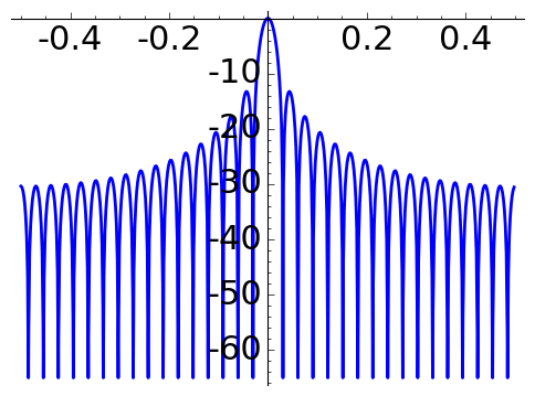
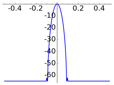
In engineering, the quality of a window is measured studying the width of the main lobe and the size of the peak side lobe in the attenuation in decibels \[A(x)= 20\log_{10}\Big|\frac{f(x)}{f(0)}\Big|.\]
The following plots of \(A\) for \(N=16\) are obtained with the code below.
|
Rectangular window |
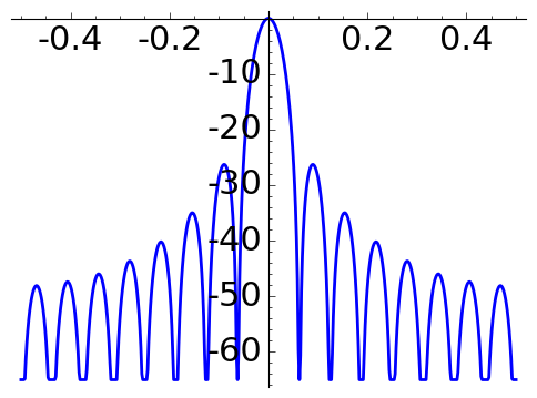 |
Triangular window |
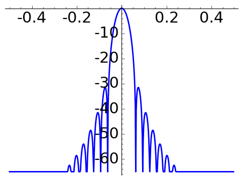 |
Hann window |
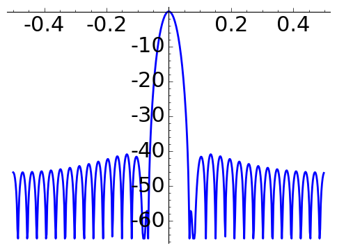 |
Hamming window |
 |
Blackman window |
N = 16 |