Windowed transforms


We consider a function essentially consisting in two peaks at ±5/2.

twopeaks


The actual formula es exp(-32*(x-5/2)^2)/4+exp(-32*(x+5/2)^2)/4.

We first analyze it using a Gabor transform, a normalization of exp(-(lambda*x)^2/2).


For lambda = 8 this window should be optimal in some sense because matches perfectly the details we want to analyze. This is the contour plot in this case. The frequencies are in the vertical axis. The code is included below.

wft0
lambda = 8

And for other values of lambda (we only plot the zone around 5/2 by the symmetry):

wft1
wft2
wft3
wft4
lambda = 2 lambda = 4
lambda = 7
lambda = 12


Now we consider the wavelet transform with the Mexican hat wavelet. To compare the plots, we put in the inverse of the scale in the vertical axis.
wt0

We also repeat the plot for 1/a limited to values greater than some values because the large values corresponding to 1/a-> 0 mask the rest of the values when distributing the contour levels. This gives an idea about the variation of these levels.


wt0half
wt1
wt2
wt3
1/a > 2
1/a > 1 1/a > 0.5 1/a > 0.25


The code

The plots were done with the following sagemath codes. I did not spend time in writing elegant code.


SAGE code for the windowed Fourier transform (Gabor)
d = 5/2

g = var('g')
assume(g>0)


fk = exp(-32*x^2)/4

f = fk(x = x-d) + fk(x = x+d)

P = plot(f, x, -2*d+1,2*d-1, thickness=3)
P.fontsize(25)
P.save('../images/twopeaks.png')

b = var('b')
xi = var('xi')

f1 = f*cos(2*pi*x*xi)*exp(-g*(x-b)^2)*(2*g/pi)^(1/4)
f2 = f*sin(2*pi*x*xi)*exp(-g*(x-b)^2)*(2*g/pi)^(1/4)

reG = integral(f1, x, -oo, oo)
imG = integral(f2, x, -oo, oo)


la = 8
vg = la^2/2
print sqrt(2*vg)
ff = -sqrt( (reG(g=vg))^2 + (imG(g=vg))^2 )

P = contour_plot(ff, (b,-4,4), (xi,0,5), plot_points=300, contours=10, linewidths=0)
P.set_aspect_ratio(1)
P.fontsize(25)
P.save('../images/wft0.png')


la = [2,4,7,12]
for k in srange(4):
vg = la[k]^2/2
print sqrt(2*vg)
ff = -sqrt( (reG(g=vg))^2 + (imG(g=vg))^2 )
P = contour_plot(ff, (b,1,4), (xi,0,5), plot_points=300, contours=10, linewidths=0, ticks=[[1.5, 2.5, 3.5],None])
P.set_aspect_ratio(1)
P.fontsize(25)
P.save('../images/wft'+str(k+1)+'.png')


SAGE code for the wavelet transform
a = var('a')
b = var('b')
assume(a<>0)

mh = (1-x^2)*exp(-x^2/2)/sqrt(2*pi)

mhft = (2*pi)^2*x^2*exp(-2*pi^2*x^2)
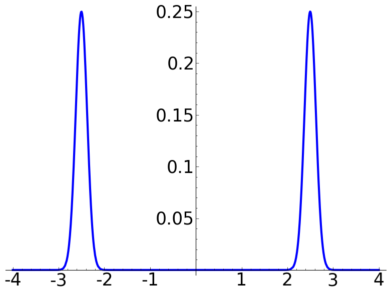
fk = exp(-32*x^2)/4

d = 5/2
f =  fk(x = x-d) + fk(x = x+d)


wt = f(x=a*x+b)*mh*sqrt(a)

wt =  sqrt(a)*(1-x^2)*exp(-x^2/2 -32*a^2*x^2 - 64*a*b*x - 32*b^2 + 160*a*x + 160*b - 200 )/sqrt(2*pi)/4
wt += sqrt(a)*(1-x^2)*exp(-x^2/2 -32*a^2*x^2 - 64*a*b*x - 32*b^2 - 160*a*x - 160*b - 200 )/sqrt(2*pi)/4

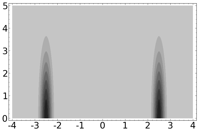
wt = integral(wt,x,-oo,oo)


wt = (wt.expand()).simplify()


ff = -abs(wt(a=1/a))


P = contour_plot(ff, (b,-4,4), (a,0,5), plot_points=300, contours=10, linewidths=0)
P.fontsize(25)
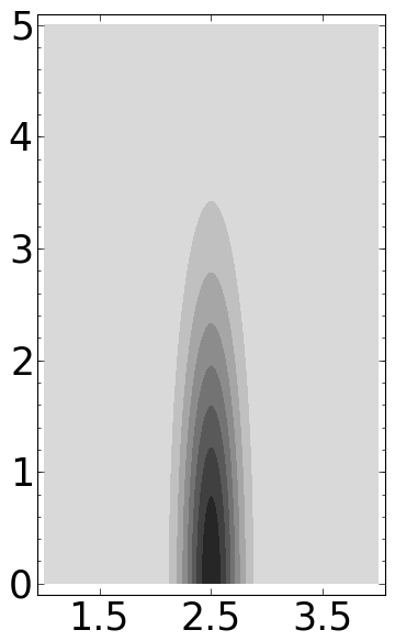
P.save('../images/wt0.png')
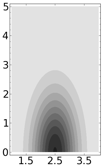
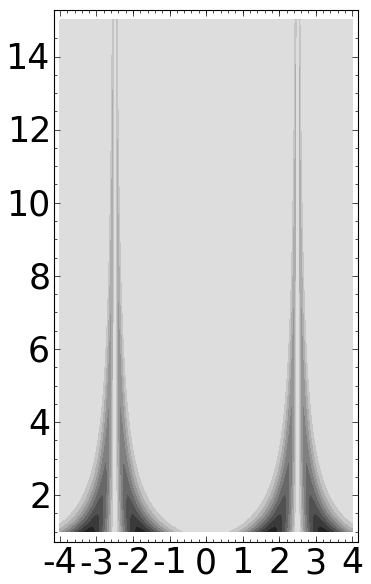
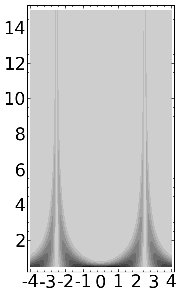
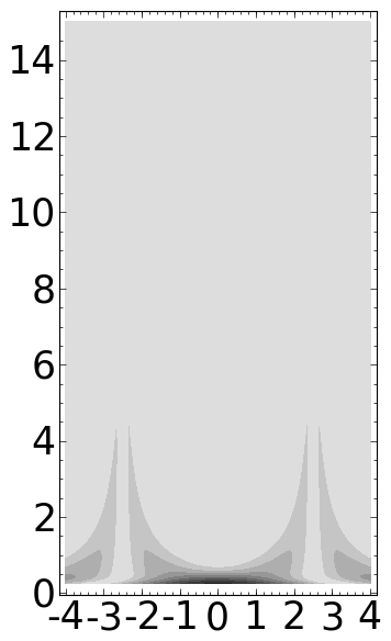
d = 5/2
wt =  sqrt(a)*(d-b)*exp(-a^2*(d-b)^2)
wt += sqrt(a)*(d+b)*exp(-a^2*(d+b)^2)
wt *= 1/sqrt(2*pi)

ff = -abs(wt)

P = contour_plot(ff, (b,-4,4), (a,2,15), plot_points=300, contours=10, linewidths=0)
P.fontsize(25)
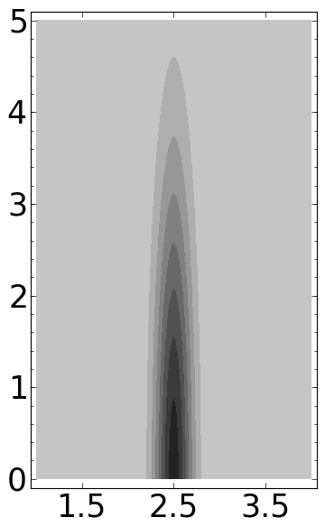
P.save('../images/wt0half.png')

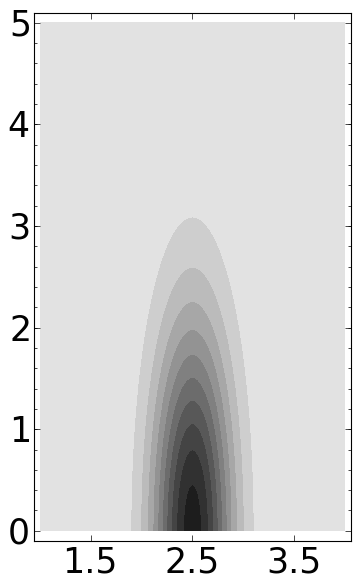
P = contour_plot(ff, (b,-4,4), (a,1,15), plot_points=300, contours=10, linewidths=0)
P.fontsize(25)
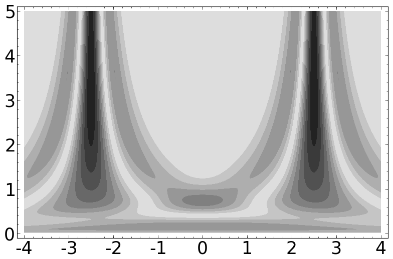
P.save('../images/wt1.png')

P = contour_plot(ff, (b,-4,4), (a,0.5,15), plot_points=300, contours=10, linewidths=0)
P.fontsize(25)
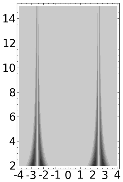
P.save('../images/wt2.png')

P = contour_plot(ff, (b,-4,4), (a,0.25,15), plot_points=300, contours=10, linewidths=0)
P.fontsize(25)
P.save('../images/wt3.png')