Lattice points in the sphere

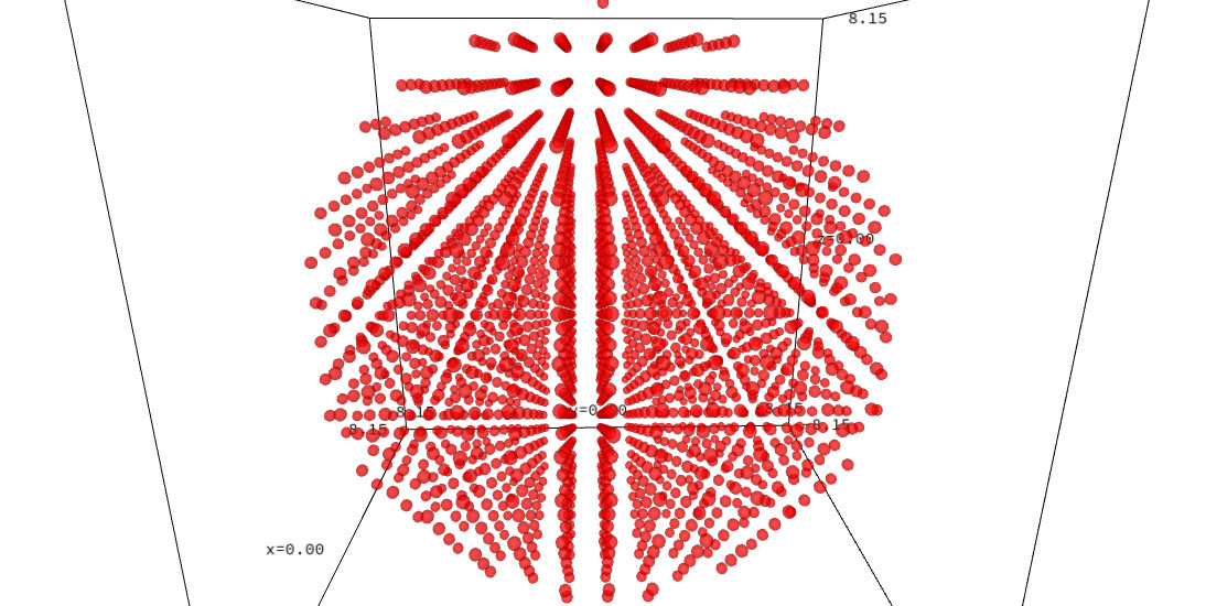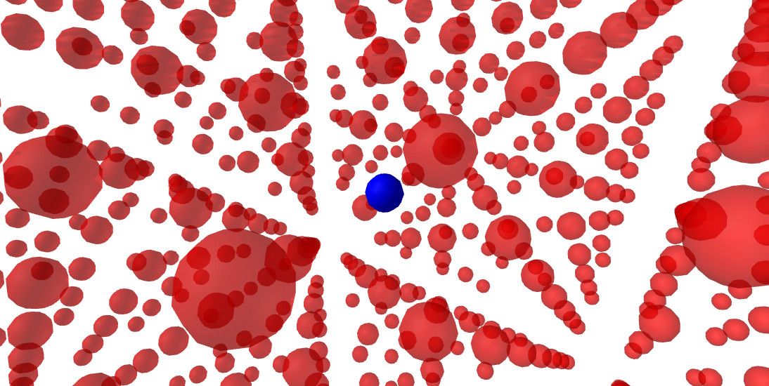
The points with integral coordinates in a large convex body approximate in some sense its shape. Here there are three views of the lattice points in a sphere of radius 8. They are colored in a semi transparent red color. These figures, as well as the rest are generated with the sagemath code below. The variation in the view point (indicated in the caption) reveals some patterns.

The figure on the left is a close-up of the patterns near the origin. The figure on the right only represent the lattice points that are visible from the origin, those having coprime coordinates.

The blue solid point is the origin.

Lattice point discrepancy for the sphere

The number of lattice points in a large convex body is well approximated by its volume. A classical problem in analytic number theory consists in studying the error in this approximation for large spheres. The results are commonly presented in the form \[\#\big\{ \vec{n}\in\mathbb{Z}^3\,:\, \|\vec{n}\|\le R \big\} = \frac{4\pi}{3}R^3 +O\big(R^{\alpha+\varepsilon}\big) \qquad\text{for every}\quad \varepsilon>0.\] It is known that necessarily \(\alpha\ge 1\) and the folklore conjecture is that \(\alpha=1\) is valid.

Let \(r_3(n)\) be the number of representations of \(n\) as sum of three squares, \(\#\big\{ \vec{n}\in\mathbb{Z}^3\,:\, \|\vec{n}\|^2=n \big\}\). Motivated by Euler-Mclaurin formula a natural variant of the error is the arithmetic function \[E(N)=\sum_{n=0}^N r_3(n)-\frac 12 r_3(N)- \frac{4\pi}{3}N^{3/2}\] It corresponds to a sphere of radius \(\sqrt{N}\) with the points on the boundary weighted by \(1/2\). These are the plots of \(E(N)\) for \(0\le N<100\) and \(0\le N<1000\)

And this is the plot for \(0\le N<10000\). In the second figure the successive maxima and the successive minima have been joined with lines.

Low frequency resonance

Formally, applying Poisson summation formula it is obtained \[E(N) = -\frac{\sqrt{N}}{\pi} \sum_{n=0}^\infty \frac{r_3(n)}{n}\cos\big(2\pi \sqrt{nN}\big) +\textrm{negligible terms}.\] The convergence of the series is unclear but it is possible to give it a sense multiplying the coefficients by a smooth function \(\varphi(n/N)\) with \(\varphi(0)=1\). In general, the quotient \(r_3(n)/n\) is larger for \(n\) small. Then one can hope some correlation between values of the cosine close to \(1\) and minima and values close to \(-1\) and maxima, for small \(n\). On the other hand, large values of \(n\) give a relevant contribution to the second power moment (this is not so in the 2D case, the Gauss circle problem), so this correlation could be not noticeable.

The six values with \(r_3(n)/n<3\) are, ordered by decreasing size of this quotient, \(n=1,2,5,6,14,9\). Let us assign them the colors red, yellow, green, cyan, blue and magenta, respectively. These figures represent the values of \(\cos\big(2\pi \sqrt{nN}\big)\) for the values of \(N\) at which the successive maxima of \(E\) (first figure) or its successive minimum (second figure) are reached.

There is not a clear correlation but, it is apparent that the first figure is mainly below zero and the second figure is mainly over zero.

Corrections on my 1995 joint paper

In the paper [ChIw] (F. Chamizo and H. Iwaniec. On the sphere problem. Rev. Mat. Iberoamericana, 11(2):417-429, 1995) in which the exponent \(29/22\) is proved for the sphere problem there are some mistakes. They do not affect to the result and I suspect that they were just copy-paste errors coming from previous versions. I typed the paper with vi on a UNIX machine and it was my first experience with that editor. No integrated TeX editors under UNIX were available at that time.

In the bounds in the bottom part of [ChIw, p. 427] the (less important) term \(R^{5/16}\) coming from the range \(N_1\le R\) is forgotten in the range for \(R<N_1\le H^{-2}\) and it also affects to \(N_2\) because in principle (but not in the optimization), \(R\) and \(H^{-2}\) could be close. More relevant is that, as it was kindly pointed by Professor Kuba, the last term appearing in the second bound contains exponents that lack coherence with (5.3), they do not appear there. A way of solving both issues with a neat short proof is to substitute the two last estimates by \[ \max\big( N_1^{-1}V_{N_1}, H^{-1}N_2^{-3/2+\varepsilon}V_{N_2}\big) \ll \mathcal{B} \qquad\text{for}\quad R<N_1\le H^{-2}\le N_2\] where \(\mathcal{B} = \big( H^{-1/2}+R^{5/16}+R^{3/8}H^{1/8} \big) H^{-\varepsilon}\).

Let us see how to prove this inequality. Note that under \(N>R\) the term \(R^{7/24}N^{49/48}\) in Lemma 3.1 of [ChIw] is absorbed by \(R^{5/24}N^{53/48}\) getting \[N^{-1}V_N \ll N^{1/4+\epsilon} + N^{\epsilon} \min\big(R^{3/8}N^{-1/16}+R^{1/8}N^{1/16},R^{5/24}N^{5/48}\big).\] If \(N\le R^2\) then \(R^{3/8}N^{-1/16}\ge R^{1/8}N^{1/16}\) and this proves \(N_1^{-1}V_{N_1}\ll\mathcal{B}\) for \(R<N_1\le \min\big(H^{-2},R^2\big)\). This bound also holds in the range \(R^2<N_1<H^{-2}\) because \(R^{5/24}N^{5/48}=(R^2/N)^{5/48}N^{5/24}\le (H^{-2})^{5/24}\) which is absorbed by \(H^{-1/2}\). To conclude the proof of the inequality, note that the bound for \(N^{-3/2}V_N\) provided by Lemma 3.1 of [ChIw] decreases in \(N\), then \(N_2^{-3/2}V_{N_2}\) can be bounded by the same estimate as that for \(N_1^{-1}V_{N_1}\) with \(N_1=H^{-2}\) multiplied by \((H^{-2})^{-1/2}\).

Beside these corrections, in the first gluing variables step there is a lack of explanations. If one applies Lemma 2.2 of [BoIw] (E. Bombieri and H. Iwaniec. On the order of \(\zeta(1/2+it)\). Ann. Scuola Norm. Sup. Pisa Cl. Sci. (4), 13(3):449-472, 1986) as indicated, then \(\theta\) may depend on \(n\) and we cannot proceed with the second step. We need a two dimensional version of this result to rule out this dependence.

If \(I\) is an interval, \(M\in \mathbb{Z}_{\ge 0}\) and \(f\) is a function with \(f(I)\subset [0,M]\), consider a subset of \(\mathbb{Z}^2\) of the form \(\mathcal{D} = \big\{ (n,m)\in\mathbb{Z}^2\,:\, n\in I,\ 0\le m\le f(n) \big\}\). Instead of [BoIw,Lemma 2.2], we apply the following one with a similar proof.

Lemma. For any \(a_{nm}\in\mathbb{C}\), there exists \(\theta\in\mathbb{R}\) such that \[\Big| \sum_{(n,m)\in\mathcal{D}} a_{nm} \Big| \le 3\log(M+2) \sum_{n\in I} \Big| \sum_{m=0}^M a_{nm} e(m\theta) \Big|.\]

Proof. For each \(n\) consider \(\chi_n(x) = \max\big( \min(1, x+1, \lfloor f(n)\rfloor+1-x), 0\big)\), a piecewise linear regularization of the characteristic function of \(\big[0, \lfloor f(n)\rfloor\big]\). Its Fourier transform satisfies \(\big|\widehat{\chi}_n(\theta)\big|\le K(\theta)\) where \(K\) is the \(n\) independent kernel \(K(\theta)=\min\big(M+1,|\pi\theta|^{-1},|\pi\theta|^{-2}\big)\). It follows easily from the trivial estimate \(\big|\widehat{\chi}_n(\theta)\big|\le M+1\) and the exact representation (integrate by parts) \[2\pi i \theta\widehat{\chi}_n(\theta) = \int_{-1}^0 e(-\theta x)\; dx - \int_{\lfloor f(n)\rfloor}^{\lfloor f(n)\rfloor+1} e(-\theta x)\; dx.\] Then \[\Big| \sum_{(n,m)\in\mathcal{D}} a_{nm} \Big| = \Big| \int_{-\infty}^\infty \sum_{n\in I}\sum_{m=0}^M \widehat{\chi}_n(\theta) e(\theta m)a_{nm}\; d\theta \Big| \le \Big| \sum_{(n,m)\in\mathcal{D}} a_{nm} \Big| \le \|K\|_1 \sum_{n\in I} \Big| \sum_{m=0}^M a_{nm} e(m\theta) \Big|\] for some \(\theta\in \mathbb{R}\). The value of \(\|K\|_1\) is explicitly given by \[\begin{aligned} \|K\|_1 = 2\int_0^\infty K &= 2\int_0^{\theta_0}(M+1)\; d\theta + \frac{2}{\pi} \int_{\theta_0}^1\frac{d\theta}{\theta} + \frac{2}{\pi^2} \int_{1}^\infty\frac{d\theta}{\theta^2} \qquad\text{with } \theta_0=\frac{1}{\pi(M+1)} \\ &= \frac{2}{\pi}\big( 1+\log\pi +\pi^{-1}+\log(M+1) \big) \end{aligned}\] and it is smaller than \(3\log(M+2).\ \square\)

The code


def r2fact(m):

  if m<0: return 0

  if m<2: return 3*m+1

  L = list(factor(m))

  res = 4

  for item in L:

    if Mod(item[0],4)==3 and is_odd(item[1]): return 0

    if Mod(item[0],4)==1: res *= item[1]+1

  

  return res

  



from sage.plot.plot3d.shapes import *

r = 0.15

Rad = 8

S = Sphere(r, color='blue')

for k1 in srange(-Rad,Rad+1):

    for k2 in srange(-Rad,Rad+1):

        for k3 in srange(-Rad,Rad+1):

            if k1^2+k2^2+k3^2>Rad^2 or k1^2+k2^2+k3^2==0: continue

            # Uncomment for visible points

#            if gcd([k1,k2,k3])>1: continue

            S += Sphere(r, color='red',opacity=0.5).translate(k1,k2,k3)

            

S.aspect_ratio(1)

S.frame_aspect_ratio(1)

# uncomment one of them

S.show(iewer='tachyon')

# S.show(iewer='tachyon', frame = False, axes = False)

  

  

  

N = 10000

Lrep2 = [r2fact(m) for m in srange(N)]



Lrep3 = N*[0]

Nsqr = ceil(sqrt(N))





# m = k1^2+k^2+(\pm j)^2

for j in srange(1,Nsqr):

  for m in srange(j^2, N):

    # 2 is for \pm j

    Lrep3[m] += 2*Lrep2[m-j^2]

#contribution of j = 0 (third square = 0)

for m in srange(0, N): Lrep3[m] += Lrep2[m]

    

E = [0.5]

for k in srange(1,N):

  res = E[-1] + Lrep3[k-1]/2 + Lrep3[k]/2 +4*pi/3*( (k-1)^(3/2)-k^(3/2) )

  E.append(res.n())



  

for k in [100, 1000, 10000]:

  P = list_plot(E[:k])

  P.save('./sph_e_'+str(k)+'.png')



# Indexes of the maxima

Limaxp = [0]

imaxp = 0

Limaxn = [0]

imaxn = 0

for k in srange(1,N):

  if E[k] <  E[imaxp]:

    imaxp = k

    Limaxp.append(k)

  if E[k] >  E[imaxn]:

    imaxn = k

    Limaxn.append(k)

    

P += line( [(ind,E[ind]) for ind in Limaxp], color='red', thickness=2 )

P += line( [(ind,E[ind]) for ind in Limaxn], color='green', thickness=2 )

P.save('./sph_e_10000_Mm.png')





Lfreq = [1,2,5,6,14,9]

stp = 460

# red, yellow, green, cyan, blue, magenta

col = rainbow(len(Lfreq))

Pp = point([(0,0),(0,1/2)], size=0)

Pn = point([(0,0),(0,1/2)], size=0)

for k in srange(len(Lfreq)):

  Pp += line([(ind,cos(2*pi*sqrt(Lfreq[k]*ind))) for ind in Limaxp if ind>stp], rgbcolor=col[k], thickness=2)

  Pn += line([(ind,cos(2*pi*sqrt(Lfreq[k]*ind))) for ind in Limaxn if ind>stp], rgbcolor=col[k], thickness=2)

Pp.save('./sph_c_p.png', figsize=[8,4])

Pn.save('./sph_c_n.png', figsize=[8,4])


camera\(\scriptsize=[25.8444,18.7771,18.4437]\)	camera\(\scriptsize=[-0.8169,0.3234,20.9632]\)	camera\(\scriptsize=[-19.9983,0.457,6.3315]\)
viewpoint\(\scriptsize=[-0.2469,-0.4845,-0.8392],133.7\)	viewpoint\(\scriptsize=[-0.0142,0.0209,0.9997],111.62\)	viewpoint\(\scriptsize=[-0.5001,0.5117,0.6986],111.35\)