Petr's miracle

In the always interesting Mathologer channel there is a video about what it is called there Petr's miracle, a nice geometrical result that was unnoticed by the mathematical community during many years and still today is not widely known.

The statement, proof and several details can be checked in the video or in the wikipedia entry about Petr-Douglas-Neumann theorem. The purpose here is to show some examples and provide my own code to produce them. In connection with this, the figures in this document are generated with the sagemath code below. Full resolution versions are obtained clicking on the images.

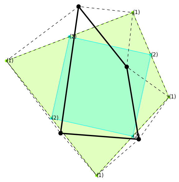
The result is a generalization of Napoleon's theorem that can be rephrased saying that when we place isosceles triangles with apex angles of 120 degrees on the sides of a given triangle then the apex vertices, marked with (1) in the figure, determine an equilateral triangle (in green color). In the usual statement, the isosceles triangles are assumed to be drawn on the exterior of the given triangle.

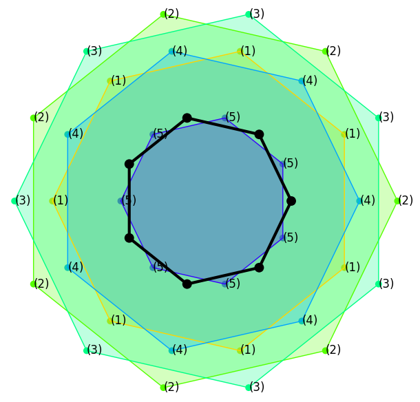
Petr's miracle, Petr-Douglas-Neumann theorem, generalizes the result to polygons of n sides. Isosceles triangles with apex vertexes of 360/n degrees are employed to produce a first generation of apex vertexes that determine a new n-gon. The second generation is obtained from the first one using apex angles of 360·2/n and the process is iterated using angles of 360·k/n degrees in the k-step until the n-2 generation of apex vertexes that, magically, determine a regular n-gon.

For quadrilaterals, n=4, the angles for the first generation are right angles and for the second generation are straight angles leading to degenerate triangles (segments with the apex vertex on the middle point).

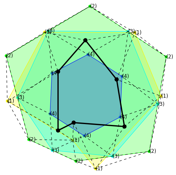
For n greater than 4 in high generations they appear reflex angles (greater than 180 degrees). This is interpreted drawing the isosceles triangles in the other side, invading the interior part. Notice in the following example for n=6 the lines connecting the vertexes of the third generation (3) with those of the fourth (4). In this case the angles are of 240 degrees and correspond to triangles as in Napoleon's theorem (of 120 degrees apex angle) but towards the interior part.

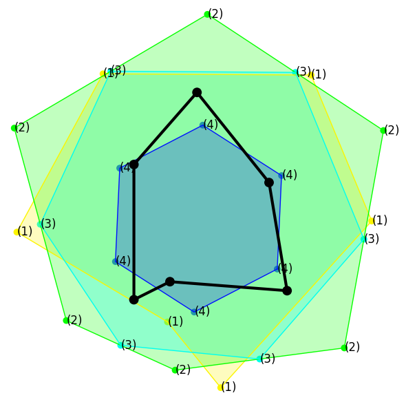
As exemplified in the previous figure, the result works for non convex polygons. The funny thing is that it also works for arbitrary polygonal lines even if they do not determine a simple polygon.

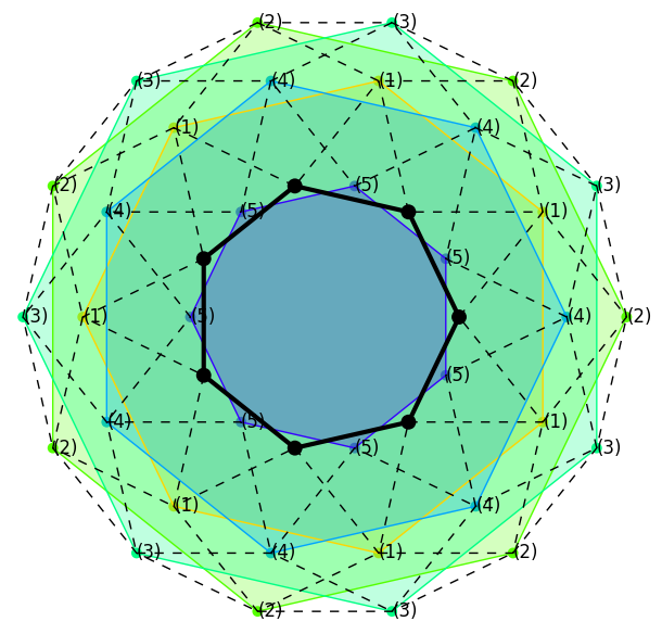
This situation in which there are not clearly defined interior and exterior regions, leads to questions about at what side the isosceles triangles should be placed. Summing up, once an orientation is fixed, there is a well defined right side and a left side when we walk around the polygonal line. See the details in the video.

One of the proofs of the result (the one in the previous video) is based on noticing that regular polygons are eigenpolygons, so to speak, of the process. They only suffer rotations and dilations. This is an example with n=7:

Some experiments show that the process mollifies in some sense the irregularities. In the next figure we see that attaching a nose to the previous heptagon it becomes less prominent in the second generation and in the fourth generation we observe an almost regular polygon.

The code


def ppol(L,k):

  Lpo = [ (real(itez),imag(itez)) for itez in L]

  if k==0:

    P = line( Lpo + [Lpo[0]] , thickness = 3, color = 'black', zorder = 100 )

    P += points(Lpo, color = 'black', size=100*s, zorder = 100)

    return P

  cm = colormaps.hsv

  col = cm(floor(k*255/len(L)))[:3]

  P = points(Lpo, color = col, size=50*s)

  P += polygon(Lpo,color = col, alpha = 0.25)

  P += line(Lpo+[Lpo[0]],color = col, zorder=80)

  for v in range(len(L)):

    P +=  text('('+str(k)+')',Lpo[v], horizontal_alignment='left', fontsize = 12, color= 'black', zorder = 100)

  return P

  

def petrit(L,k):

  ph = exp(2*pi*i*k/len(L))

  M = L + [L[0]]

  return [ ((M[k+1]-ph*M[k])/(1-ph)).n() for k in range(len(L))]



def pconnect(L,Ln):

  Lpo1 = [ (real(itez),imag(itez)) for itez in L] + [ (real(L[0]),imag(L[0]))]

  Lpo2 = [ (real(itez),imag(itez)) for itez in Ln]

  P = point([Lpo1[0]],size=0)

  for k in srange( len(L) ):

    P += line([Lpo1[k+1], Lpo2[k], Lpo1[k]], color='black', zorder=100, linestyle='--')

  return P

  

def petr(L, co = True):

  L.reverse()

  P = ppol(L,0)

  for k in srange(1, len(L)-1):

    Ln = petrit(L,k)

    if co: P += pconnect(L,Ln)

    P += ppol(Ln,k)

    L = Ln[:]

  P.axes(False)

  P.set_aspect_ratio(1)

  return P

  

  

s = 1 # scale



L = [0, 8/7-i/10, 1+i]

P = petr(L)

P.save('./petr_3.png')  # triangle



L =[-0.1-0.1*i, 1.2-0.2*i, 1+i, 0.2+2*i]

P = petr(L)

P.save('./petr_4.png')  # quadrilateral



L = [-1, 0.2+2*i, 0.3-i, 1+0.7*i, -0.8-3*i/2, 0.4+1.5*i]

P = petr(L, False)

P.save('./petr_ns.png')  # not simple



L = [exp(2*pi*i*k/7) for k in srange(7)]

P = petr(L, False)

P.save('./petr_7r.png')  # regular heptagon



L = [exp(2*pi*i*k/7) for k in srange(7)]

P = petr(L)

P.save('./petr_7rc.png')  # regular heptagon connection lines



L = [exp(2*pi*i*k/7) for k in srange(7)]

L[0] = 3+i

P = petr(L, False)

P.save('./petr_7.png')  # heptagon with nose



L =[-0.5+1.2*i, -0.5-0.3*i, -0.1-0.1*i, 1.2-0.2*i, 1+i, 0.2+2*i]

P = petr(L)

P.save('./petr_6c.png')  # non convex hexagon connection lines



L =[-0.5+1.2*i, -0.5-0.3*i, -0.1-0.1*i, 1.2-0.2*i, 1+i, 0.2+2*i]

P = petr(L,False)

P.save('./petr_6.png')  # non convex hexagon