The Parks-McClellan algorithm is an approach based on the
alternation theorem
for the design of optimal FIR filters.
Here we test the algorithm as implemented in matlab to construct a low-pass filter with passband [0,7/40] and stopband [9/40,1/2].
We consider in the
matlab code the cases
delta=0.09,
delta=0.017 and
delta=0.004
that with the notation in my signal processing course corresponds to
N=7,
N=16 and
N=24.
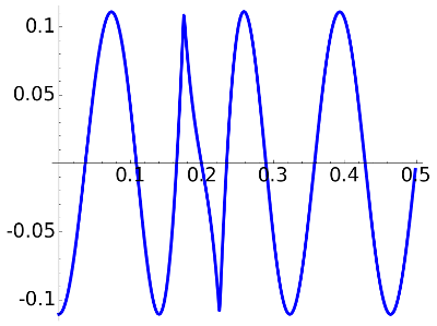
First of all let us see the graph of the approximated filter in comparison with the ideal low-pass filter with a linear behavior in the transition band.
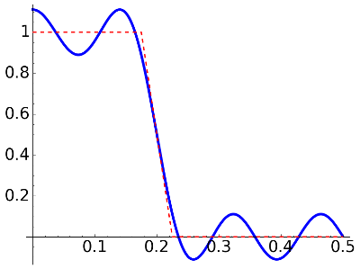 |
delta=0.09, N=7
|
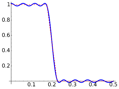 |
delta=0.017, N=16
|
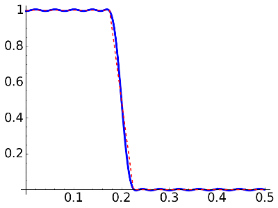 |
delta=0.004, N=24
|
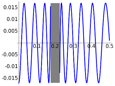
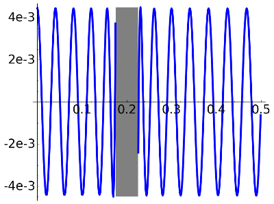
According to the numerical data, the maximal errors in the passband and the stopband are
0.11076,
0.016955 and
0.0045000 which are close to the specified values of delta. The plots of the errors in these zones is
 |
delta=0.09, N=7
|
 |
delta=0.017, N=16
|
 |
delta=0.004, N=24
|
This is in clear agreement with the expected equioscillation property.
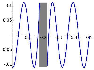
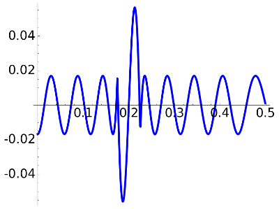
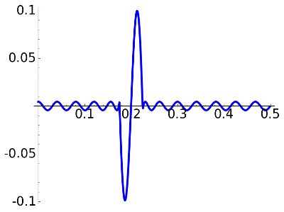
If you are curious about the aspect of the graphs of the error including the transition band, here they are:
 |
delta=0.09, N=7
|
 |
delta=0.017, N=16
|
 |
delta=0.004, N=24
|
The code
This is the matlab code that generates the data. Uncomment the lines with % to see some figures.
df = 0.025;

nuc = 0.2;

delta = 0.09;


passb = nuc-df;

stopb = nuc+df;

dpass = delta;

dstop = delta;

nusamp = 1;


[n,fo,ao,w] = firpmord([passb stopb],[1 0],[dpass dstop],nusamp);

b = firpm(n,fo,ao,w);

[h,w] = freqz(b,1,512);

%figure(1)

%plot(fo/2,ao,w/pi/2,abs(h));


kv = [0:511]';

newh = h.*exp(n*pi*i/1024*kv);

%figure(2)

%plot(fo/2,ao,w/pi/2,real(newh));

%figure(3)

%plot(w/pi/2,real(newh));

format shortE

%size(real(newh))


disp('------------------------------------------')

disp((n-1)/2)

delta

%real(newh)
The data generated putting in the matlab program the different values of delta
was stored in files
dpm1.txt,
dpm2.txt,
dpm3.txt
and the figures above were generated with the following SAGE program:
for k in srange(1,4):

  with open('dpm'+str(k)+'.txt','r') as f:

    text = f.read()


    temp = text.split('\n')[:512]

    for m in srange(512):

      temp[m] = sage_eval( temp[m] )


    P = line( [(0,1),(7/40,1),(9/40,0), (1/2,0)], thickness=2, linestyle='--', color='red', zorder= 60)

    P += list_plot([(m/1024,temp[m]) for m in srange(512)], plotjoined=True, thickness=4)

    P.fontsize(25)

    P.save('./pa_mc_'+str(k)+'.png')


    error = [(m/1024,1-temp[m]) for m in srange(180)]

    error += [( m/1024, 20*(9/40-m/1024)-temp[m]  ) for m in srange(180, 231)]

    error += [( m/1024,0-temp[m] ) for m in srange(231, 512)]

    P = list_plot( error, plotjoined=True, thickness=4)

    P.fontsize(25)

    P.save('./pa_mc_er'+str(k)+'.png')


    error = [(m/1024,1-temp[m]) for m in srange(180)]

    P = list_plot( error, plotjoined=True, thickness=4)

    ma = 1-min(temp[:180])

    mi = 1-max(temp[:180])

    error = [( m/1024,0-temp[m] ) for m in srange(231, 512)]

    ma = max( ma, 0-min(temp[231:512]) )

    mi = min( mi, 0-max(temp[231:512]) )


    print k,'->',max(-mi,ma)

    P += list_plot( error, plotjoined=True, thickness=4)


    P += plot( ma+0*x,7/40,9/40, fill=mi+0*x, color='gray', fillcolor='gray', fillalpha=1)

#    P += polygon([(7/40,ma), (9/40,ma), (9/40,mi), (7/40,mi)], color='gray')


    P.fontsize(25)

    P.save('./pa_mc_e'+str(k)+'.png')