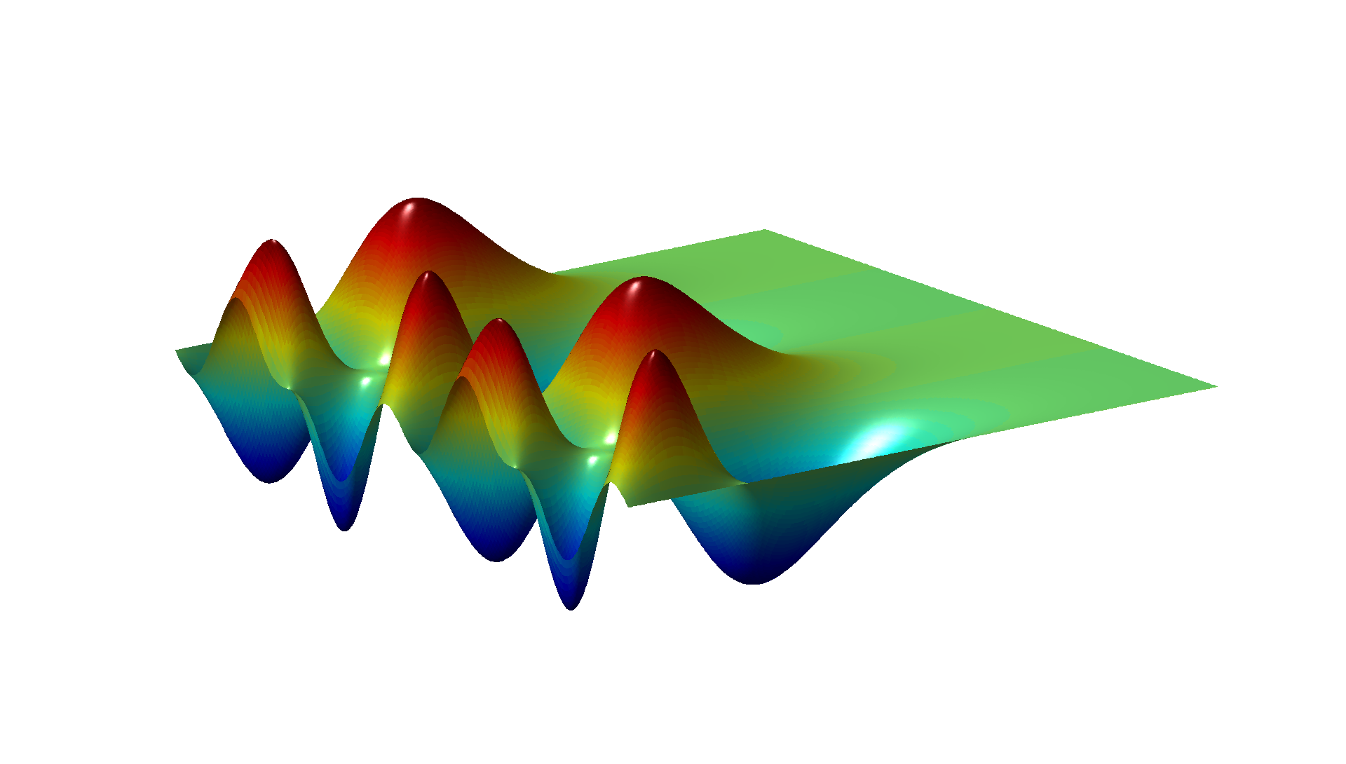
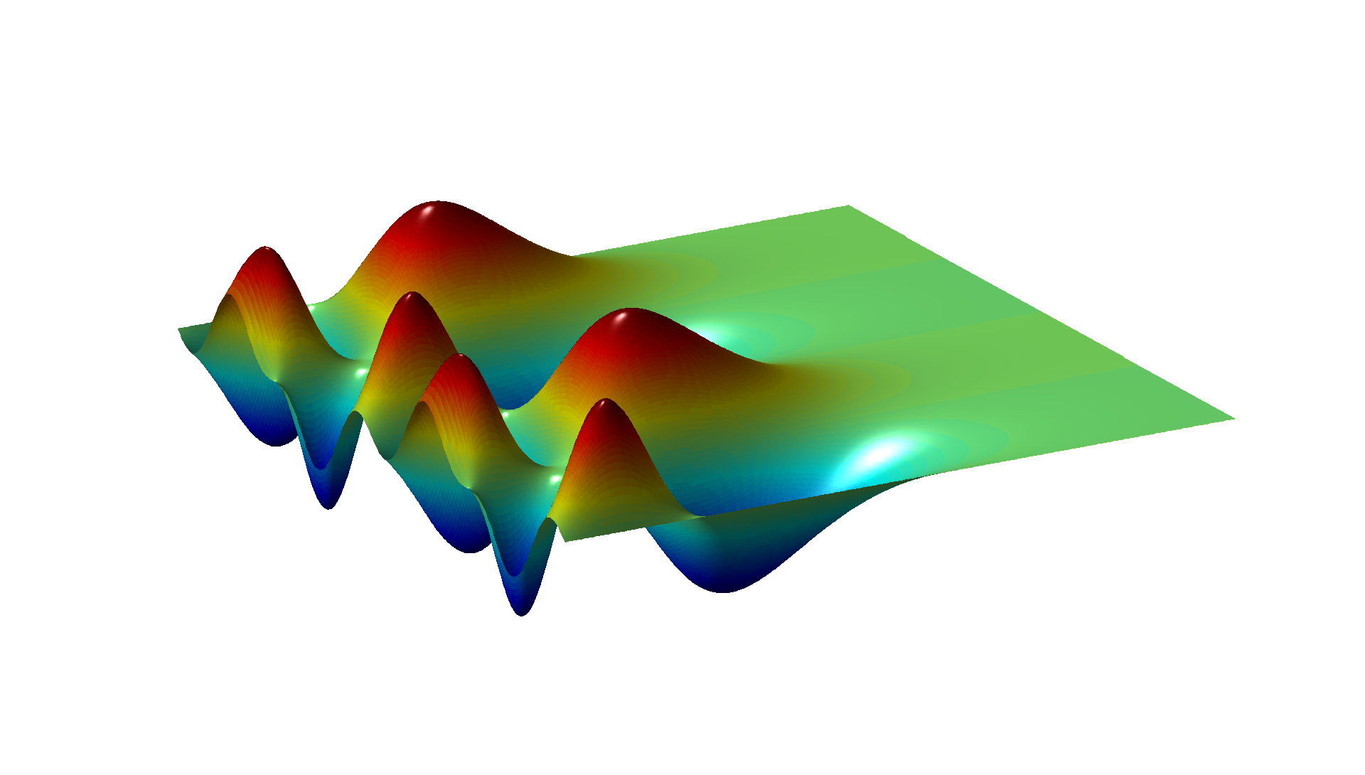
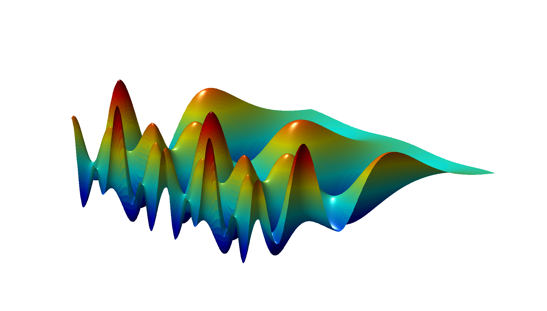
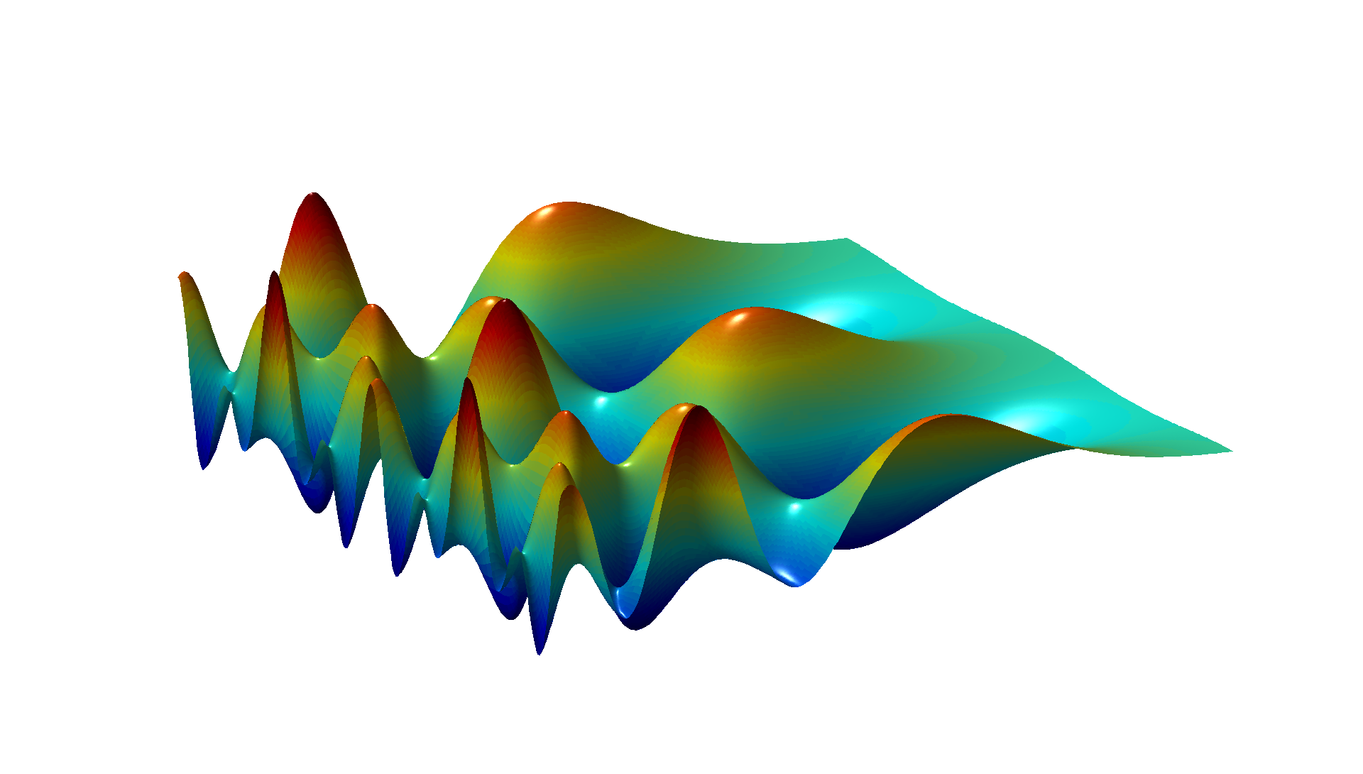
The first Maass cusp form for SL2(Z)
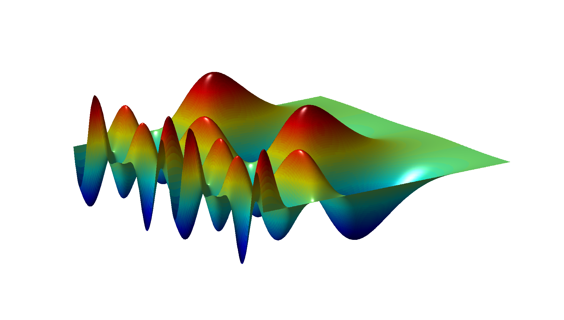
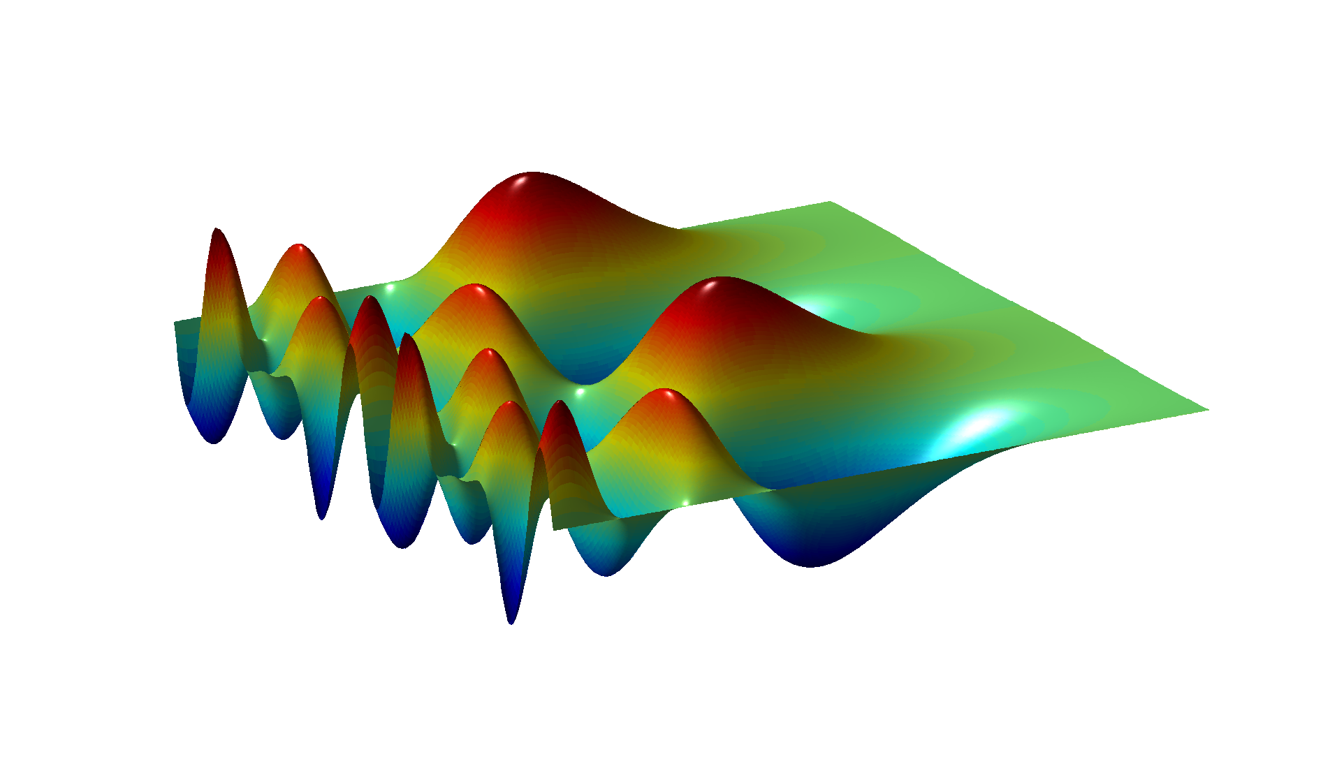
The second Maass cusp form
The third Maass cusp form
In these plots -1<x<1 and 0.5<y<3. The left and right figures only differ in the angle of the view.
The code
A cheap way of plotting an approximation of the Maass form is using the
first terms in the Fourier expansion. It requires computing Bessel
function with imaginary argument. This can be done with SAGE. We also
have to know the corresponding eigenvalue (1/4+t^2) and the Fourier
coefficients that can be taken from here or here. Since Octave/Matlab plots finely 3D functions, I have used the following SAGE
code to generate three Octave/Matlab tables containing the data:
###########################################

# MAKE ku1_def.m, ku2_def.m, ku3_def.m #

# WITH THE VALUES OF THE K-BESSEL IN u_j #

###########################################


# number of y in the range [0.5,3]

N = 300


def make_kuj_def(j,t,a):
    file = open("ku"+str(j)+"_def.m", "w")
    # HEADER
    file.write("KU"+str(j)+" = [ ")


    for k2 in range(N):
        y = (2.5*k2/N+0.5).n()
        L = 7*[0.0];

        k = 0
        while ((2*pi*k*y)<30) and (k<7):

            k += 1
            L[k-1] = (a[k]*real(bessel_K(I*t,
(2*pi*k*y)))*exp(pi*t/2)*sqrt(y)).n()
        # print to file
        for k in range(6):
            file.write(str(L[k])+',')
        file.write(str(L[6]))
        if k2==N-1:
            file.write(str( ']'))
        file.write(str( ';\n'))
    file.close()


#######################################

# u1 eigenvalue with t = 9.53369526135

#######################################

t = 9.53369526135

a = [0, 1, -1.0683335512, -0.45619735450, 0.14133657666, -0.2906725549,
0.4873709397983, -0.7449416121475798]

make_kuj_def(1,t,a)


#######################################

# u2
eigenvalue with t = 12.173008324679677
#######################################
t = 12.173008324679677
a = [0, 1, 0.28925187146, -1.201858761, -0.91633335485,
0.039552707287414, -0.347639895856, 0.4481331044912988]
make_kuj_def(2,t,a)
#######################################
# u3 eigenvalue with t = 13.779751351890738
#######################################
t = 13.779751351890738
a = [0, 1, 1.54930447794, 0.2468997724, 1.40034436536, 0.737060385348,
0.382522923065639, -0.26142007576521]
make_kuj_def(3,t,a)
And I run the following Matlab code to plot the data. Octave does not
admit exactly the same options (at least in the version I use).
%%%%%%%%%%%%%%%%%%%%%%%%%%%%%%%%


%% RUN FIRST bess_matlab.sage %%


%%%%%%%%%%%%%%%%%%%%%%%%%%%%%%%%


%%%%%%%%%%%%%

% PLOT u1 %

%%%%%%%%%%%%%


% load data

ku1_def;

N = size(KU1,1);


% meshgrid for u1

U1 = KU1*sin(2*pi*[1:7]'*fliplr(linspace(-1,1, N)));


% plot

figure(1)

surf(linspace(0.5,3, N),linspace(-1,1, N),U1','EdgeColor','none')

colormap jet

camlight left; lighting phong

axis off


% plot

figure(2)

surf(linspace(0.5,3, N),linspace(-1,1, N),U1','EdgeColor','none')

colormap jet

camlight left; lighting phong

view([-30,40])

axis off


%%%%%%%%%%%%%

% PLOT u2 %

%%%%%%%%%%%%%


% load data

ku2_def;

N = size(KU2,1);


% meshgrid for u2

U2 = KU2*sin(2*pi*[1:7]'*fliplr(linspace(-1,1, N)));


% plot

figure(3)

surf(linspace(0.5,3, N),linspace(-1,1, N),U2','EdgeColor','none')

colormap jet

camlight left; lighting phong

axis off


% plot

figure(4)

surf(linspace(0.5,3, N),linspace(-1,1, N),U2','EdgeColor','none')

colormap jet

camlight left; lighting phong

view([-30,40])

axis off


%%%%%%%%%%%%%

% PLOT u3 %

%%%%%%%%%%%%%


% load data

ku3_def;

N = size(KU3,1);


% meshgrid for u3

U3 = KU3*cos(2*pi*[1:7]'*linspace(-1,1, N));


% plot

figure(5)

surf(linspace(0.5,3, N),linspace(-1,1, N),U3','EdgeColor','none')

colormap jet

camlight left; lighting phong

axis off


% plot

figure(6)

surf(linspace(0.5,3, N),linspace(-1,1, N),U3','EdgeColor','none')

colormap jet

camlight left; lighting phong

view([-30,40])

axis off