|
def plot_spline(Y):
# Make spline matrix
N = len(Y)-1
A = 4.0*identity_matrix(N+1)
A += block_matrix([[ 0, identity_matrix(N) ], [ zero_matrix(1,1), 0 ]])
A += block_matrix([[ 0, zero_matrix(1,1) ], [ identity_matrix(N), 0 ]])
A[0,0] = 2
A[N,N] = 2
############################
#solve
b = vector( Y[1:N+1]+[Y[N]] )
b -= vector( [Y[0]]+Y[0:N] )
d = A.solve_right(3*b)
d = list(d)
############################
# plot
P = point([(0,Y[0])],size=0)
P += list_plot(list((j/N,Y[j]) for j in srange(N+1)), size=100)
for j in range(N):
s1 = d[j+1]+d[j]-2*(Y[j+1]-Y[j])
s2 = -d[j+1]-2*d[j]+3*(Y[j+1]-Y[j])
P += plot( s1*(N*x-j)^3+s2*(N*x-j)^2+d[j]*(N*x-j)+Y[j], x, j/N,(j+1)/N, thickness=3)
return P
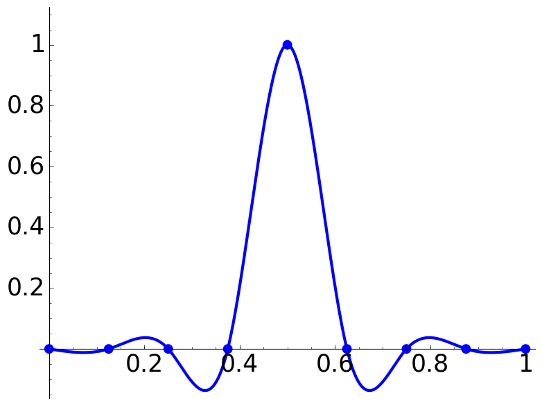
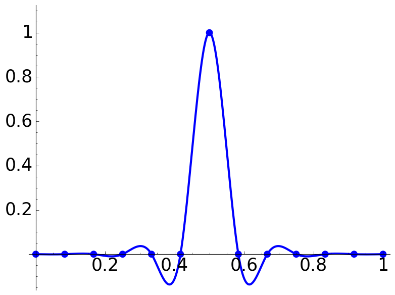
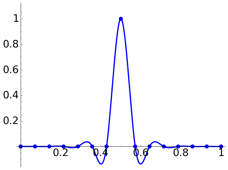
K = 7
he = 1.0
L = K*[0]+[he]+K*[0]
P = plot_spline(L) + point([(0,he*1.1)],size=0)
P.fontsize(25)
#P.set_aspect_ratio(1)
#P.axes(False)
P.show()
|