Let \(F\) be a B/W \(M\times N\) image. This means that we have a function \[F:\{0,\dots, M-1\}\times \{0,\dots, N-1\}\longrightarrow [0,1]\] where \(F(m,n)\) is the tone of gray (0=black, 1=white) of the pixel \((m,n)\).
The illumination-reflectance model claims that for an artistic photo we can factorize \(F=IR\) where \(I\) gives the illumination that contains low frequencies and \(R\) gives the reflectance that contains higher frequencies. Sometimes, when we take a photo a part is poorly illuminated and the result is not very pleasant (unless you are Caravaggio!). According to the previous model, the solution is to replace \(I\) by a constant giving to the photo a uniform illumination. The problem is how to obtain this theoretical factorization. We can overcome this point taking \(\log F\) and wiping out the low frequencies with Fourier analysis. In this way \(\log I\) disappears and with an exponential we obtain \(R\) that gives the image with the uniform illumination \(I=1\). This procedure is called homomorphic filtering. The strange name is related to the property of the logarithm as a homomorphism taking products into sums.
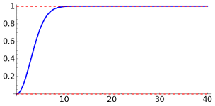
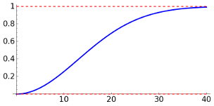
To avoid complex numbers, I will use here the DCT instead of the DFT. The method to eliminate the low frequencies is to consider a high-pass filter given by the operator \[H = \text{DCT}^{-1}(G\cdot \text{DCT}).\] Ideally, \(G\) should take the value 0 on a centered circle and 1 elsewhere but this sharp cut can produce artifacts (recall the Gibbs phenomenon) and on the other hand the model does not establish a clear difference between low and high frequencies. In practice, they are preferred functions of the form \[G(m,n) = (\gamma_H-\gamma_L) \Big( 1-\exp\big(-\frac{m^2+n^2}{2\sigma^2}\big) \Big)+\gamma_L\] for some parameters \(\gamma_L\), \(\gamma_H\) and \(\sigma\). The most natural choice is \(\gamma_L=0\), \(\gamma_H=1\). The following graphs show the radial profile of \(G\) in this case for two values of \(\sigma\), which indicates in some sense the level of smoothing.
|
|
|
| \(\sigma=3\) | \(\sigma=30\) |
Another practical issue is that \(\log F\) does not make sense if \(F\) vanishes at some point (if there are black pixels) and also small values of \(F\) can affect the result. It suggests to replace \(F\) by \(F+\epsilon\) with \(\epsilon\) a small constant. Summing up, we apply homomorphic filtering in the form \[F \longmapsto \exp\big( (H\circ\log)(F+\epsilon) \big)-\epsilon.\]
To play with an example, I took a photo of a curves page looking for inducing a shadow and I got the following \(512\times 512\) not evenly illuminated result, unfortunately some faint symbols from the back page are slightly visible. Probably a better example would be an artistic image with gradients instead of a text but I did not have any poorly illuminated example at hand. Then we stick to
 |
| Original image |
The octave code below applies the homomorphic filtering with \(\epsilon=1/512\) and different choices of the parameters. It also applies the ideal high-pass filter. In this case \(G\) firstly 1 exactly on a circle of radius 20 and the result is
 |
| Ideal high-pass filter \(r=20\) |
 |
| Ideal high-pass filter \(r=40\) |
The instances of the not ideal case displayed by the program are:
 |
| \(\sigma=60\), \(\gamma_L=0\) and \(\gamma_H=1\) |
 |
| \(\sigma=30\), \(\gamma_L=0\) and \(\gamma_H=1.1\) |
Finally, if we increase too much \(\gamma_H\) we have still a better contrast, which is good for a text but also a noise of high frequencies to the right is exaggerated and the result is not very satisfactory.
 |
| \(\sigma=60\), \(\gamma_L=0\) and \(\gamma_H=3\) |
This is the octave code that implements homomorphic filtering and produces the figures:
pkg load image

pkg load signal


clear all


ima = imread('../images/pages3.png');

ima = im2double(ima);


epsi = 1/256/2;


% Ideal high-pass

r = [20,40];

[X, Y] = meshgrid(1:size(ima,1), 1:size(ima,2));

rsq = X.^2 + Y.^2;

for k=1:2

  H = (rsq>r(k)^2);

  In = idct2(H.*dct2(log(epsi + ima)));

  res = exp(In) - epsi;

  imwrite( min( max( res, 0), 1) , sprintf('./homp_%d.png',k));

end


param = [60,0,1; 30, 0, 1.1; 60, 0, 3]

for k = 1:size(param,2)

  namef = sprintf('./hom_f%d.png',k);

  hom_ff( ima, param(k,1), param(k,2), param(k,3), epsi, namef)

end


% All the results are clipped
It calls the following function:
% Apply  homomorphic filtering with parameters sig, gL, gH to the square image ima with epsilon = epsi and saves the result in fname


function hom_ff( ima, sig, gL, gH, epsi, fname)

  [X, Y] = meshgrid(1:size(ima,1), 1:size(ima,2));

  rsq = X.^2 + Y.^2;


  H = (gH-gL)*(1-exp(-rsq/2/sig^2))+gL;

  In = idct2(H.*dct2(log(epsi + ima)));

  res = exp(In) - epsi;

  imwrite( min( max( res, 0), 1) ,fname);

end
The following SAGE code was employed to plot the two radial profiles of \(G\).
def plotg( sigma, a,b ):

  gH = 1

  gL = 0

  H = (gH-gL)*(1-exp(-x^2/2/sigma^2))+gL;

  P = plot( H,x, a,b, thickness=3)

  P += line([(a,0),(b,0)], thickness=2, zorder=40, linestyle='--', color='red')

  P += line([(a,1),(b,1)], thickness=2, zorder=40, linestyle='--', color='red')

  return P


P = plotg( 3, 0,40 )

P.fontsize(20)

P.save( 'hom_g1.png', figsize=[8,4] )


P = plotg( 13, 0,40 )

P.fontsize(20)

P.save( 'hom_g2.png', figsize=[8,4] )