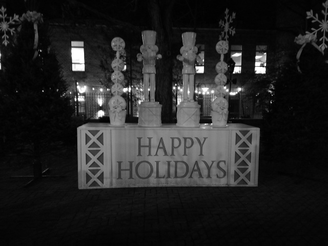
We are going to consider three actions on the histograms of a couple of images to enhance them.
Our first test image is the following photo. It was taken by night. The lights in the background saturates the white and the details in the foreground are hidden in similar gray tones.
 |
| Original image 1 |
The second test image is out of focus (but we do no not treat this problem here) and shows no contrast between the paper and the surface.
 |
| Original image 2 |
These are the histograms of the images. In both cases they are essentially concentrated in a part of the interval [0,1]. In the first case there are tiny bars near 1, representing the white spots.
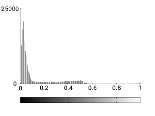 | 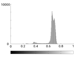 |
| Histogram image 1 | Histogram image 2 |
We first apply histogram equalization as implemented in octave (see the code below). In practice it does not flatten completely the histogram because the gray levels are discrete but it distributes the values more evenly. In our case, the result is:
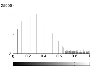 | 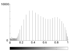 |
| Equalized histogram 1 | Equalized histogram 2 |
This equalization acts quite well in the first case to show a couple of trees difficult to see in the original.
 |
| Equalized image 1 |
On the other hand the result is bad for the second image. Some noise due to the low quality of the photo is considered as "details" and acquires the same black tone as the text.
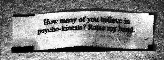 |
| Equalized image 2 |
As in both cases the histograms are rather localized, a second natural procedure is to crop the levels and stretch the histogram.
For the first image, in the code below the levels are cropped to [0, 0.6] that contains almost all the mass and the result is stretched to the whole range [0,1]. Doing this, we obtain the following image. It improves the original but we do not distinguish the hidden details.
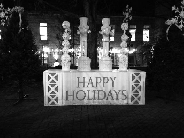 |
| Cropping-Stretching 1 |
For the second image the natural interval is [0.2,0.8]. The result improves the original and is much better than the equalization.
 |
| Cropping-Stretching 2 |
Finally, we are going to apply a logarithmic model. Basically it correspond to apply cropping and stretching to the logarithm of the values of the pixels divided by the values of a blurred version of the image (my signal processing course). In both cases we use [-1.8, 1.2] and the blurred image comes from applying a Gaussian filter with standard deviation 60.
For the first image the log model gives a result with a slightly more natural aspect than the equalization and still reveals the hidden results.
 |
| Log model for image 1 |
For the second image the result is, to my taste, a little better than the previous direct cropping and stretching.
 |
| Log model for image 2 |
This is the octave code to produce the images.
pkg load image


clear all


name = '../images/happy_r_bw.jpg'

name = '../images/cookie.jpg'


ima1 = imread( '../images/happy_r_bw.jpg' );

ima1 = im2double(ima1);


ima2 = imread( '../images/cookie.jpg' );

ima2 = im2double(ima2);


figure(1)

imhist( ima1, 256 );


figure(2)

imhist( ima2, 256 );


% Equalization

res = hist_mod( ima1, 256, 0, 0);

imwrite( res, './his_eq1.jpg' );


figure(3)

imhist( res, 256 );


res = hist_mod( ima2, 256, 0, 0);

imwrite( res, './his_eq2.jpg' );


figure(4)

imhist( res, 256 );


% Crop - Stretch

res = hist_mod( ima1, 0.0, 0.6, 1);

imwrite( res, './his_cs1.jpg' );


res = hist_mod( ima2, 0.2, 0.8, 1);

imwrite( res, './his_cs2.jpg' );


% Log model

res = hist_mod( ima1, -1.8, 1.0, 2);

imwrite( res, './his_lm1.jpg' );


res = hist_mod( ima2, -1.8, 1.0, 2);

imwrite( res, './his_lm2.jpg' );
It calls to the function hist_mod:
% Three histogram modifications in images

% ima image

% a,b parameters

% t = 0 ->equalization, a=nbins, b=arbitrary

% t = 1 ->stretching, a=min, b=max

% t = 2 ->log model, a=min, b=max (g=60, eps=1/256)


function res = hist_mod( ima, a, b, t )


  if t==0

    % Equalization

    res = histeq( ima, a );


  elseif t==1

    % Cropping-stretching

    res = max(ima, a);

    res = min(res, b);


  elseif t==2

    % log model

    res = imsmooth(ima, "Gaussian", 60);

    res = log((ima+1/256)./res);

    res = max(res, a);

    res = min(res, b);


  end


  % normalize

  res = im2double(mat2gray(res));


end