Harmonic oscillations

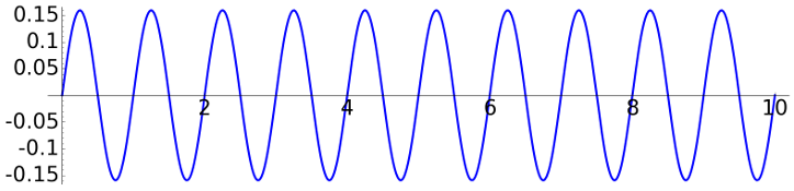
The differential equation \[x''+\omega^2x=0 \qquad\text{with}\quad x=x(t)\] rules the harmonic oscillator. This equation gives a good approximation for the motion of a particle attached to a spring or the small oscillations of a simple pendulum. For normalization we consider the initial conditions \(x(0)=0\), \(x'(0)=1\) and the solution is \[x(t)= \omega^{-1}\sin(\omega t).\]

For a fluid like air, in first approximation, the friction is proportional to the velocity (Stokes' law) and then the model equation becomes \[x''+2ax'+\omega^2x=0 \qquad\text{with}\quad a>0.\] This is the damped harmonic oscillator. If the friction is not very large, \(a<\omega\) and the solution is still oscillatory \[x(t)= \widetilde{\omega}^{-1}e^{-at}\sin(\widetilde{\omega}t) \qquad\text{with}\quad \widetilde{\omega}=\sqrt{\omega^2-a^2}.\]

If some periodic external force acts on the oscillator, by Fourier analysis we can restrict ourselves to cosines or cosines with a phase which leads to the equation of the driven harmonic oscillator \[x''+2ax'+\omega^2x=F_e\cos(\omega_e t-\varphi_e).\] Its general solution is \[x(t)=A\cos(\omega t)+B\sin(\omega t) +x_p(t)\] where \(x_p\) is the particular solution \(x_p(t)=C\cos(\omega_e t-\varphi)\) with \[C= \frac{F_e}{\sqrt{(\omega^2-\omega_e^2)^2+4a^2\omega_e^2}} \quad\text{and}\quad \varphi = \arg \Big( \frac{F_e e^{i\varphi_e}}{\omega^2-\omega_e^2-2ia\omega_e} \Big).\] This particular solution is the steady-state solution, the limit when \(t\to +\infty\) of any solution under any initial conditions. Under our initial conditions \[A = -x_p(0) \qquad\text{and}\qquad B = \widetilde{\omega}^{-1}\big(1- x_p'(0)- ax_p(0)\big).\] The denominator in \(C\) measures the gain. If \((\omega^2-\omega_e^2)^2+4a^2\omega_e^2\) is small then \(C>F_e\), the external force is amplified. This requires small friction \(a\) and \(\omega\approx \omega_e\). This is the phenomenon of resonance. If \(a\) is small but not zero, then eventually the solution stabilizes to \(x_p\) which has large amplitude. In the limit case \(a=0\) one obtains an unbounded amplitude given by a linear polynomial. For instance, for \(a=\varphi_e=0\), \(F_e=\omega=\omega_e=1\) the solution under our initial conditions is \(x(t)=(0.5t+1)\sin t\).

Let us see some examples. The figures were made with the code below.

The simplest example is of course the solution of the pure harmonic oscillator:

\(\omega = 2\pi\)

If we introduce a small friction the reduction on the amplitude seems to be linear:

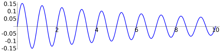\(\omega = 2\pi\), \(a=0.1\)

But, of course, it is exponential, as shown taking a more noticeable friction:

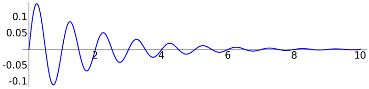\(\omega = 2\pi\), \(a=0.5\)

For a driven harmonic oscillator, if \(\omega_e\) is not close to \(\omega\), we observe a "non pure" oscillation with decreasing amplitude according to the friction. In these examples we take \(F_e=1\) and \(\varphi_e= \pi/3\).

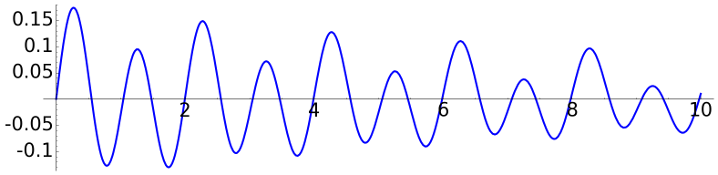\(\omega = 2\pi\), \(a=0.5\), \(\omega_e = \pi\)

We can see the phenomenon of resonance taking values approaching \(\omega\) and reducing \(a\). In this plot the black, green, blue and red lines correspond to \(\omega_e=\pi\), \(4\pi/3\), \(5\pi/3\) and \(2\pi=\omega\), respectively.

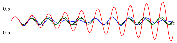\(\omega = 2\pi\), \(a=0.01\), \(\omega_e/\omega =\) \(1/2\), \(2/3\), \(5/6\), \(1\)

Taking a higher value of the friction we can notice the convergence to the steady-state solution also in the resonance case.

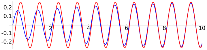\(\omega = \omega_e=2\pi\), \(a=0.3\)

The code