Clearly sagemath is not the tools for artistic drawing but for some of
us sometimes it is quicker to write a clumsy and far from optimal code
than trying our best with GIMP.
Here there are some examples (and I insist, the code is probably awful)
that are related to the electromagnetic field.
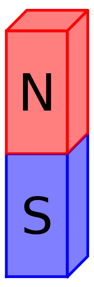
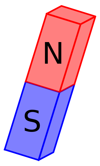
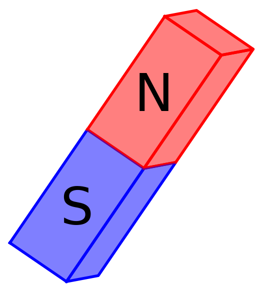
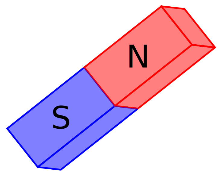
Magnets
# Magnets code --------------------------

def magneta(dx,dy,ofx,ofy, al=0):

    c = 1/3

    a = 0.5

    c1 = 'red'

    c2 = 'blue'

    L1 = [(0,0),(dx,0),(dx,dy/2),(0,dy/2),(0,0)]

    L2 = [(dx,0),(dx+c*dx,c*dx),(dx+c*dx,dy/2+c*dx),(dx,dy/2),(dx,0)]


    for L in [L1,L2]:

        for k in range(len(L)):

            L[k] = (ofx+L[k][0]*cos(al)-L[k][1]*sin(al),
ofy+L[k][0]*sin(al)+L[k][1]*cos(al) )


    P = line(L1, thickness=4, color=c2)

    P += line(L2, thickness=4, color=c2)

    P += polygon(L1, alpha=a, color=c2, zorder=5)

    P += polygon(L2, alpha=a, color=c2, zorder=5)

    for k in range(5):

        L1[k]=(L1[k][0]-dy/2*sin(al),L1[k][1]+dy/2*cos(al))

        L2[k]=(L2[k][0]-dy/2*sin(al),L2[k][1]+dy/2*cos(al))

    L3 = [(0,dy),(c*dx,dy+c*dx),(c*dx+dx,dy+c*dx),(dx,dy),(0,dy)]


    for k in range(len(L3)):

        L3[k] = (ofx+L3[k][0]*cos(al)-L3[k][1]*sin(al),
ofy+L3[k][0]*sin(al)+L3[k][1]*cos(al) )


    P += line(L1, thickness=4, color=c1)

    P += line(L2, thickness=4, color=c1)

    P += line(L3, thickness=4, color=c1)

    P += polygon(L1, alpha=a, color=c1, zorder=5)

    P += polygon(L2, alpha=a, color=c1, zorder=5)

    P += polygon(L3, alpha=a, color=c1, zorder=5)

    P
+=text("N",(ofx+dx/2*cos(al)-(dy/4+dy/2)*sin(al),ofy+dx/2*sin(al)+(dy/4+dy/2)*cos(al)),
fontsize=25*dx, color='black', zorder=20)

    P
+=text("S",(ofx+dx/2*cos(al)-dy/4*sin(al),ofy+dx/2*sin(al)+dy/4*cos(al)),
fontsize=25*dx, color='black', zorder=20)

    return P


for k in srange(4):

    P = magneta(3,12,10*k,0, -0.3*k)

    P.set_aspect_ratio(1)

    P.axes(False)

    P.save('../images/magnet'+str(k)+'.png')
# --------------------------
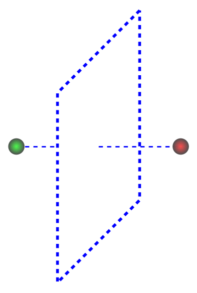
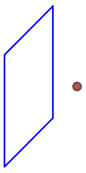
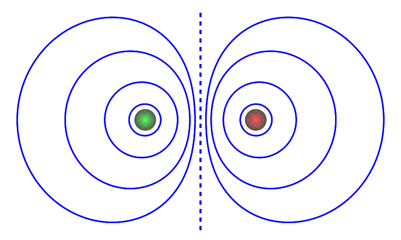
Method of images
# M. of images code --------------------------

y = var("y")

bx = 3.4

by = 2

rm = 0.2

P = point([(-1,0),(1,0)], size=0)

for r in srange(0,rm,0.01):

    P += circle( (1,0),r, rgbcolor=(1-0.7*r/rm,0.3,0.3))

    P += circle( (-1,0),r, rgbcolor=(0.3, 1-0.7*r/rm, 0.3))

f = 1/sqrt((x-1)^2+y^2)-1/sqrt((x+1)^2+y^2)

for lamb in [1,3,0.4, 0.2]:

    P += implicit_plot(f==lamb, (x, -bx, bx), (y, -by,by), ticks= [[],[]], linewidth=2)

    P += implicit_plot(f==-lamb, (x, -bx, bx), (y, -by,by), ticks= [[],[]], linewidth=2)


P += line([(0,-by),(0,by)], thickness = 3, linestyle='--')

P.axes_color('white')

P.set_aspect_ratio(1)

P.axes(False)

P.fontsize(15)

P.save('../images/mim3.png')


l = 2

h1 = 3.3

h2 = 1.3

rm = 0.2


P = point([(-l,0),(l,0)], size=0)

for r in srange(0,rm,0.01):

    P += circle( (l,0),r, rgbcolor=(1-0.7*r/rm,0.3,0.3))

    P += circle( (-l,0),r, rgbcolor=(0.3, 1-0.7*r/rm, 0.3))

P += line([(0,0),(l,0)], thickness = 2, linestyle='--')

P += line([(-l,0),(-1,0)], thickness = 2, linestyle='--')

P += line([(1,h1),(-1,h2),(-1,-h1),(1,-h2),(1,h1)], thickness = 4, linestyle='--')


P.set_aspect_ratio(1)

P.axes(False)

P.fontsize(15)

P.save('../images/mim1.png')


P = point([(l,0)], size=0)

for r in srange(0,rm,0.01):

    P += circle( (l,0),r, rgbcolor=(1-0.7*r/rm,0.3,0.3))

P += line([(1,h1),(-1,h2),(-1,-h1),(1,-h2),(1,h1)], thickness = 4)


P.set_aspect_ratio(1)

P.axes(False)

P.fontsize(15)

P.save('../images/mim2.png')
# --------------------------
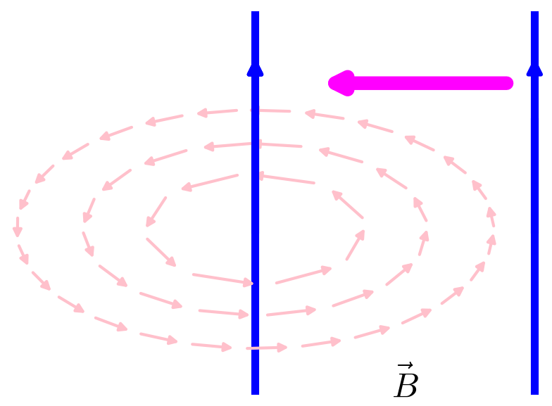
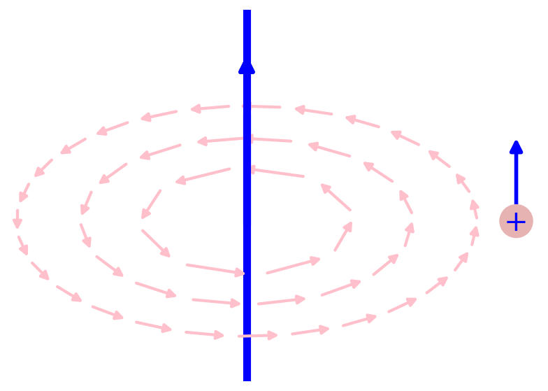
Ampère and Lorentz force laws
# A. and L. force law code --------------------------
def a_ell(r,t):
w = 0.5*(r-0.2)
h = 2*w
P = point( [(t,0)], size=0)
s1, s2 = 0.4/r^2, 0.3/r^2
for th in srange(0,2*pi,s1):
r = -0.03
x1, y1 = w*cos(th+r), h*sin(th+r)
x2, y2 = w*cos(th+s2+r), h*sin(th+s2+r)
P += arrow2d((t+y2,x2),
(t+y1,x1), width=3, arrowsize=5, color='pink', zorder=20)
P += arrow2d((t,0.7), (t,0.8), width=4, arrowsize=9,zorder=130)
return P
t = 0
P = line( [(t,0), (t,1)], thickness=8, zorder =100)
P += line( [(t,-0.75), (t,0.5)], thickness=8, zorder =0)
P += a_ell(1.31,t)
P += a_ell(1,t)
P += a_ell(0.71,t)
Q = P
P +=text('$\\vec{B}$',(0.7,-0.7), fontsize=35, color='black')
t = 1.3
P += line( [(t,0), (t,1)], thickness=8, zorder =100)
P += line( [(t,-0.75), (t,0.5)], thickness=8, zorder =0)
P += arrow2d((t,0.7), (t,0.8), width=4, arrowsize=9,zorder=130)
P += arrow2d((t*0.9,0.68), (0.3,0.68), width=14, arrowsize=9,zorder=130, color='magenta')
P.fontsize(25)
P.set_aspect_ratio(1)
P.axes(False)
P.save('../images/florentz1.png')
P = Q
t = 1.3
P += circle((t,0),0.07, thickness =5, fill = True, rgbcolor=(0.9,0.7,0.7), zorder=2)
P += text( "+", (t,0), fontsize=30, zorder=5)
P += arrow2d((t,0), (t,0.4), width=4, arrowsize=7,zorder=1)
P.fontsize(25)
P.set_aspect_ratio(1)
P.axes(False)
P.save('../images/florentz2.png')
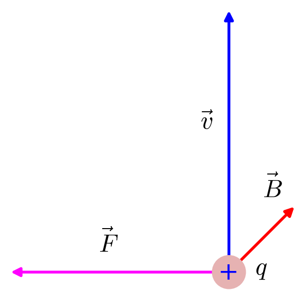
t = 1
P = circle((0,0),0.07*t, thickness =5, fill = True, rgbcolor=(0.9,0.7,0.7), zorder=2)
P += text( "+", (0,0), fontsize=35, zorder=5)
P += arrow2d((0,0), (0,1.2*t), width=4, arrowsize=7,zorder=1)
P += arrow2d((0,0), (0.3*t,0.3*t), width=4, arrowsize=7,zorder=1, color ='red')
P += arrow2d((0,0), (-1.0*t,0), width=4, arrowsize=7,zorder=1, color ='magenta')
P +=text('$\\vec{F}$',(-1.1*t/2,0.15), fontsize=35, color='black')
P +=text('$\\vec{v}$',(-0.1*t,0.7*t), fontsize=35, color='black')
P +=text('$\\vec{B}$',(0.2*t,0.4*t), fontsize=35, color='black')
P +=text('$q$',(0.15*t,0), fontsize=35, color='black')
P.fontsize(25)
P.set_aspect_ratio(1)
P.axes(False)
P.save('../images/florentz3.png')
# --------------------------
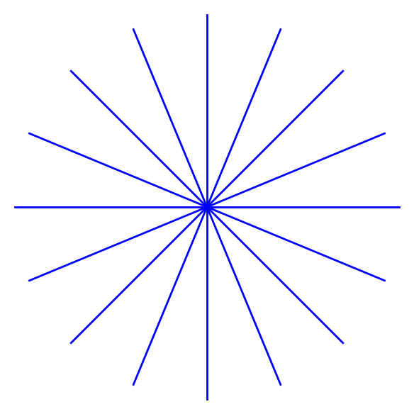
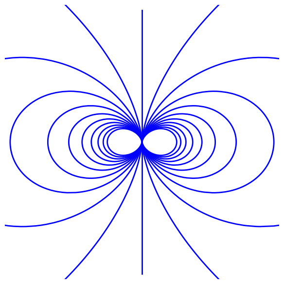
Monopole and dipoles
# Monopole and dipole code --------------------------
var ('t')
th = 2
# MONOPOLE
P = point([(0,0)])
for ang in srange(0,2*pi,2*pi/16):
P += parametric_plot( (cos(ang)*t, sin(ang)*t), (t,0,2), thickness=th)
P.xmin(-2)
P.xmax(2)
P.ymin(-2)
P.ymax(2)
P.fontsize(25)
P.set_aspect_ratio(1)
P.axes(False)
P.save('../images/flmono.png')
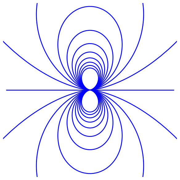
# DIPOLE
P = point([(0,0)])
for l in srange(0.1,2,0.2):
P += parametric_plot( (1/l*(sin(t))^2*cos(t), 1/l*(sin(t))^2*sin(t)), (t,0,2*pi), thickness=th)
P += parametric_plot( (t,0), (t,-2,2), thickness=th)
P.xmin(-2)
P.xmax(2)
P.ymin(-2)
P.ymax(2)
P.fontsize(25)
P.set_aspect_ratio(1)
P.axes(False)
P.save('../images/fldipo.png')
# DIPOLE 2
P = point([(0,0)])
for l in srange(0.1,2,0.2):
P += parametric_plot( (1/l*(sin(t))^2*sin(t), 1/l*(sin(t))^2*cos(t)), (t,0,2*pi), thickness=th)
P += parametric_plot( (0,t), (t,-2,2), thickness=th)
P.xmin(-2)
P.xmax(2)
P.ymin(-2)
P.ymax(2)
P.fontsize(25)
P.set_aspect_ratio(1)
P.axes(False)
P.save('../images/fldipo2.png')
# --------------------------