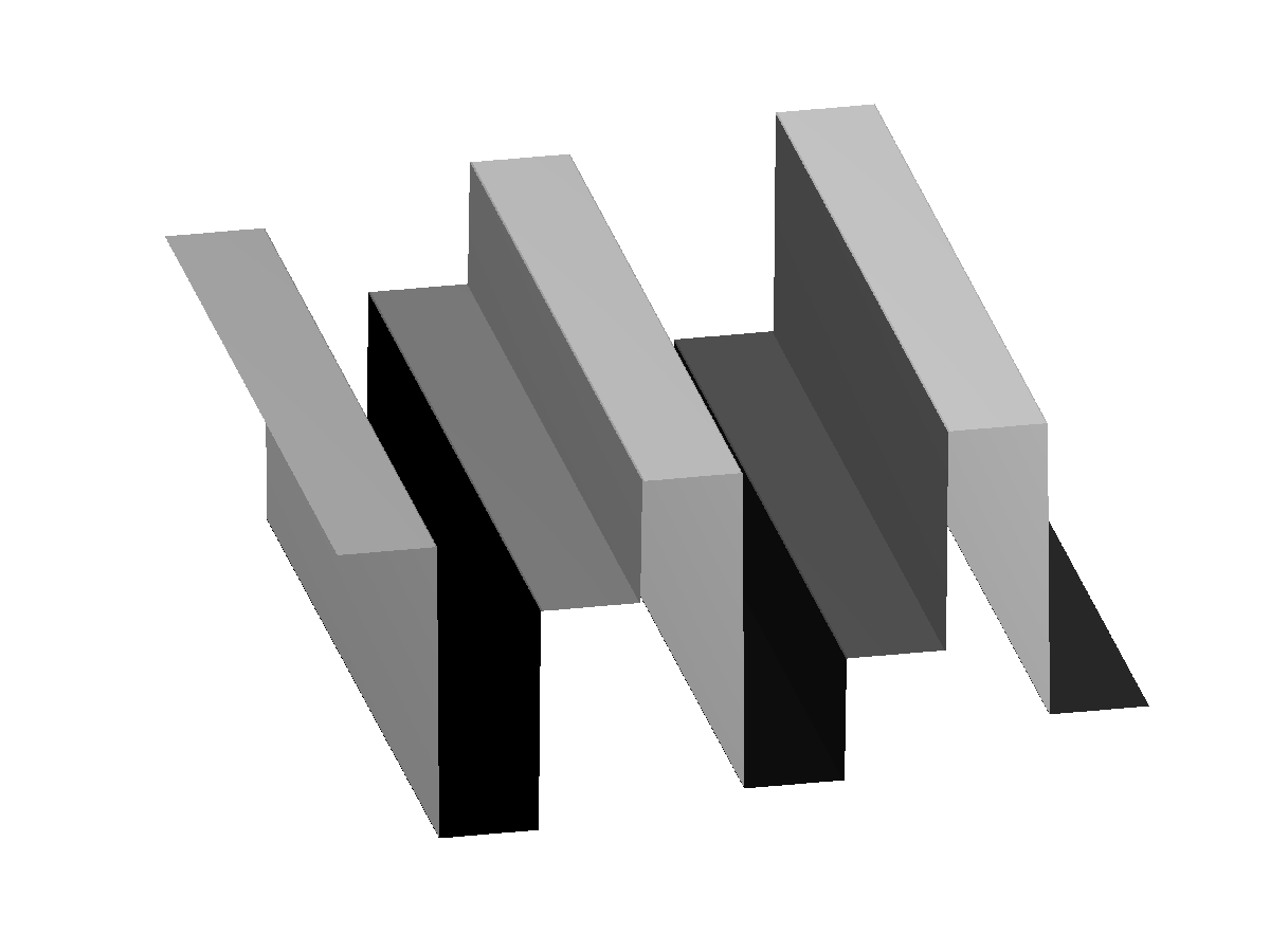
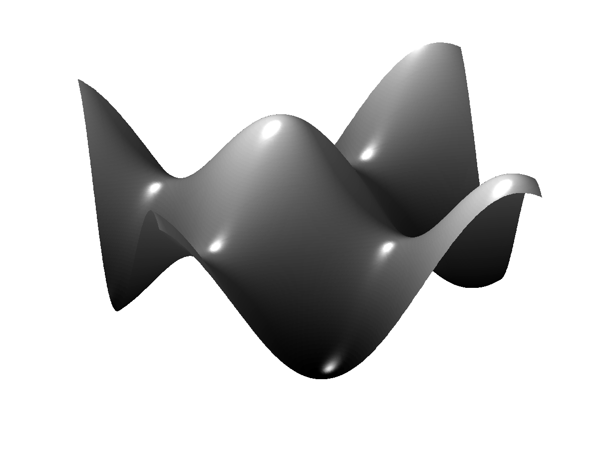
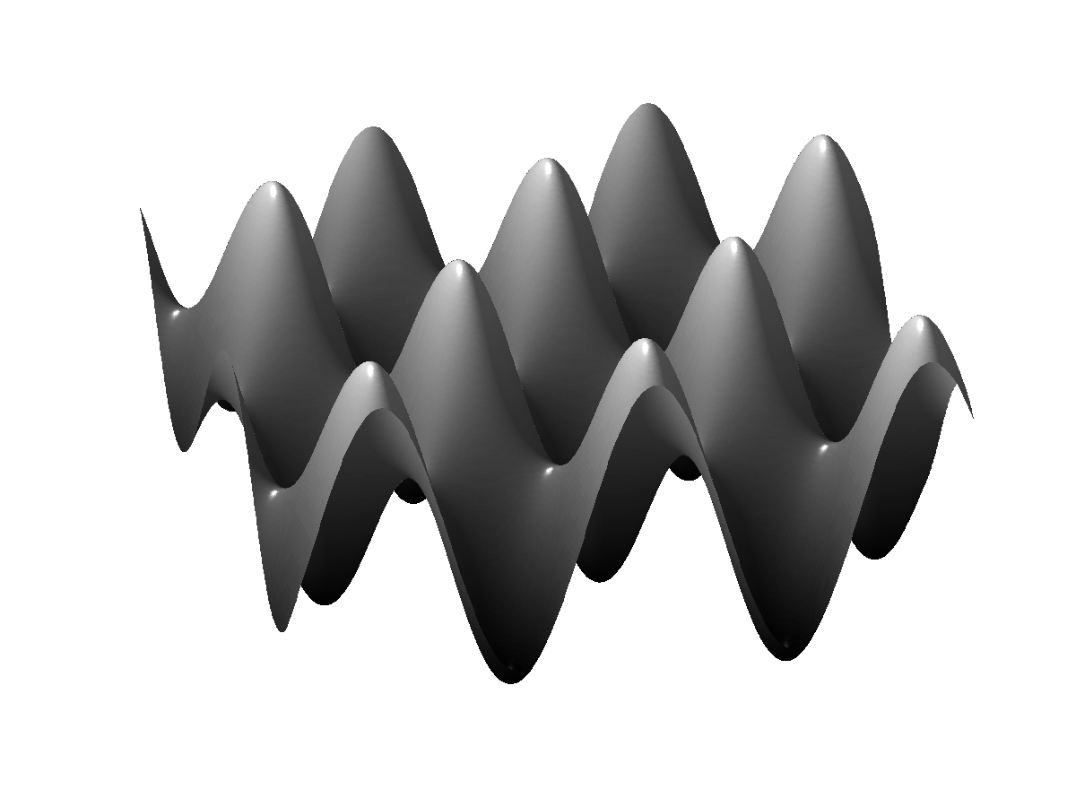
The code below, plots with Matlab (for Octave one has to do some modifications) the functions fk(x)fl(x) with fk(x)=cos(pi
k (x+1/2)/N). these are, up to a normalization, the basis functions of
DCT-II. In the code one can choose legoh=1 and legov = N to produce the
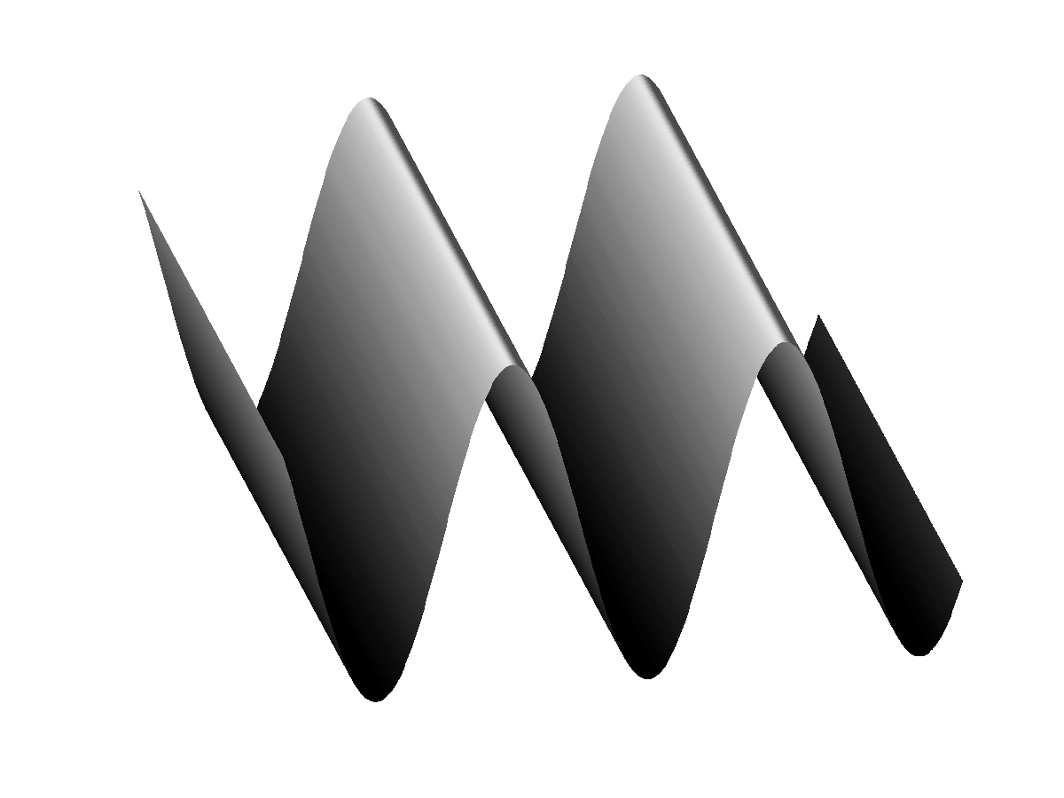
actual step functions. With large value we have approximations of the
continuous versions.
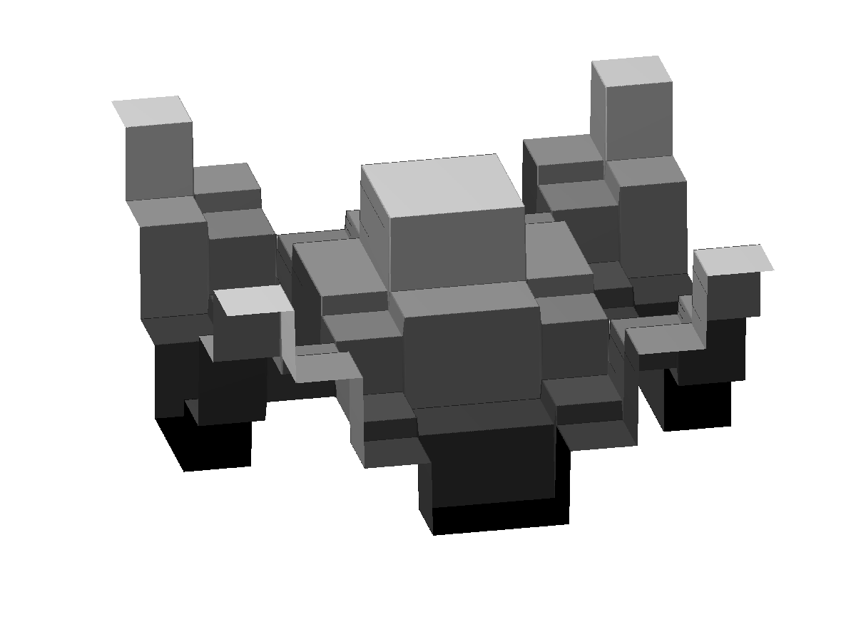
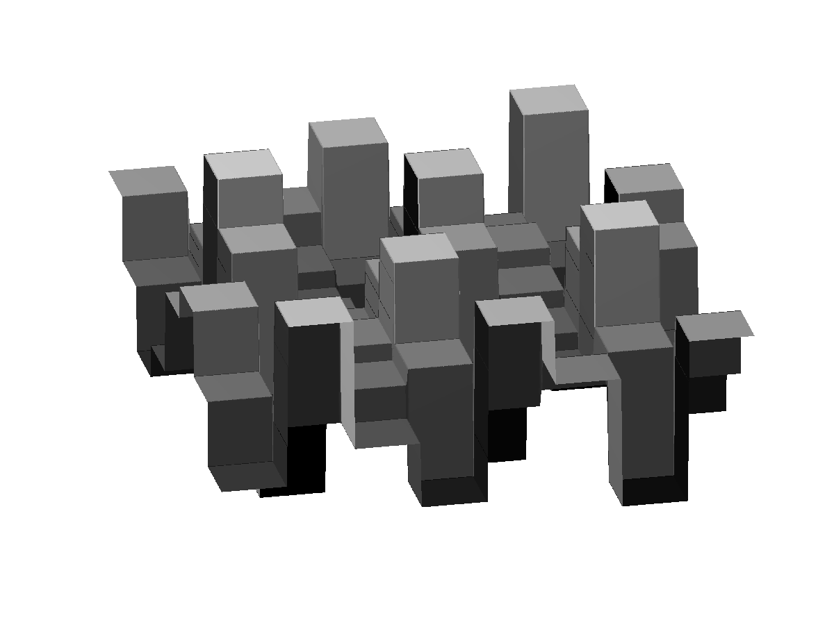
For instance, for N=8, that corresponds to JPEG, we have
k=0, l=5
|
k=2, l=2
|
k=3, l=5
|
|
 |
 |
k=0, l=5
|
k=2, l=2
|
k=3, l=5
|
|
 |
 |
The code
% DCT-II

N = 8


legoh = 1*1000;

legov = N*1000;


% meshgrid for Z

npoints = 400;

x = linspace(0,N, npoints);

y = linspace(0,N, npoints);

[X,Y] = meshgrid(x,y);


for l=0:N-1

    for k=0:N-1

        Z = cos(pi*k/2/N*(2*floor(legoh*X)/legoh+1)).*cos(pi*l/2/N*(2*floor(legoh*Y)/legoh+1));

        Z = floor(legov*Z)/legov;


        % plot

        figure(1)

        surf(X,Y,Z,'EdgeColor','none')

        colormap gray

        camlight right; lighting phong

        view([78,40])

        axis off


        namefig = './images/fig%d%d.png';

        namefig = sprintf(namefig,k,l);

        saveas(gcf,namefig)

    end

end
Other interesting values for the azimuth and elevation in view are
view([-30,40])
view([80,60])
view([66,40])
view([58,36])
view([78,28])